06.30.2005 10:40
Sun compiler issues
One of the Sun blade 100's hard disk
bought the farm recently (these machine are trouble). Once Sun put
a new disk in it and it was built back up, it's main use as the
workstation for the drafting table style digitizer was put to use,
accept that the program stopped working.
 ./digimap
ld.so.1: ./digimap: fatal: libF77.so.4: open failed: No such file or directory
Killed
Ouch. No Fortran 77 library!?!?! Checking out the program on another machine tells me where this library should live:
ldd digimapIf you do not install the compilers on every machine, then you run into troubles! How strange to not just put the lib[FM]77.so.* on every install. The solution is to install the compilers. We paid for them, but it is just another thing to have to install. The os info:
libF77.so.4 => /opt/SUNWspro/lib/libF77.so.4 libM77.so.2 => /opt/SUNWspro/lib/libM77.so.2 libsunmath.so.1 => /opt/SUNWspro/lib/libsunmath.so.1 libm.so.1 => /opt/SUNWspro/lib/libm.so.1 libc.so.1 => /usr/lib/libc.so.1 libdl.so.1 => /usr/lib/libdl.so.1 /usr/platform/SUNW,Sun-Blade-100/lib/libc_psr.so.1
uname -s -r


SunOS 5.8
06.30.2005 09:49
LaTeX AGU better style
agu-tex-snapshot.tar.bz2
This snapshot is stuff Lisa gave me yesterday for working with pdflatex. My paper suddently looks much more professional. Nice! Thanks Lisa! This puts the paper in 2 column mode and does a better job with authors.
The fron of my paper looks a little different now:
I had an idea the might help editing. What if I have mypaper.tex.in? In that file, I put a @PARAGRAPH_COUNT@ at the beginning of each paragraph. Then I write a little python script to process the .tex.in into a .tex file with each paragraph count marker replaced with the paragraph number? Something like this:
This snapshot is stuff Lisa gave me yesterday for working with pdflatex. My paper suddently looks much more professional. Nice! Thanks Lisa! This puts the paper in 2 column mode and does a better job with authors.
The fron of my paper looks a little different now:
\documentclass[agupp]{aguplus}
\usepackage{graphicx}


\def\arar {$^{40}$Ar/$^{39}$Ar }


\let\cross=\times\lefthead{Schwehr et al.}
\righthead{Santa Barbara AMS - draft $Revision:$ $Date:$ \today}


\begin{document}


\title{Title of the paper}


\author {Kurt Schwehr, Neal Driscoll, Lisa Tauxe}
\affil{Scripps Institution of Oceanography, University of California, San Diego}


\date{$Revision:$ for G-cubed}


\authoraddress{
K. Schwehr,  Scripps Institution of Oceanography,
  La Jolla,CA 92093-0220, USA (e-mail: schwerhr@gmail.com);
N. Driscoll,
  Scripps Institution of Oceanography,
  La Jolla,CA 92093-0220, USA (e-mail: ltauxe@ucsd.edu);
L. Tauxe,
  Scripps Institution of Oceanography,
  La Jolla,CA 92093-0220, USA (e-mail: ndriscoll@ucsd.edu);
}


\begin{abstract}
This is the abstract.
\begin{verbatim}
$Id: mypaper.tex,v 1.25 2005/06/29 22:22:19 schwehr Exp $
\end{verbatim}
\end{abstract}


\begin{article}
\section {Introduction}


Talk until I am blue in the face.
...


\section{Discussion}


\section{Conclusions}


Witty memorable statements go here.


% this uses mypaper.bib
\bibliography{mypaper}
\bibliographystyle{agu}
\end{article}


%======================================================================
%======================================================================
%======================================================================


\begin{figure}
\includegraphics{Figures2/core6}
\caption{ Say something insightful here.
}
\label{fig:core6}
\end{figure}


\end{document}
\end
That is the rough layout of the paper. To make the paper, here is
what I run:
  pdflatex mypaper.tex
  bibtex mypaper.aux
  pdflatex mypaper.tex
  open mypaper.pdf
Happy writing!
I had an idea the might help editing. What if I have mypaper.tex.in? In that file, I put a @PARAGRAPH_COUNT@ at the beginning of each paragraph. Then I write a little python script to process the .tex.in into a .tex file with each paragraph count marker replaced with the paragraph number? Something like this:
foo.tex.in: @PARAGRAPH_COUNT@The first paragraph.I am sure there is a way to do this in latex/tex, but I am not going to try to figure out how when I can just use python with line.find('@PARAGRAPH_COUNT@'). Unless someone wants to tell me the latex solution
@PARAGRAPH_COUNT@Another paragraph yammering on.
@PARAGRAPH_COUNT@The end.
numberParagraphs foo.tex.in foo.tex
foo.tex: [1] The first paragraph.
[2] Another paragraph yammering on.
[3] The end.
06.29.2005 20:34
MER update from Squires
http://athena.cornell.edu/news/mubss/
- The latest from Squires. I can't believe these rovers are doing
so well. I have spent so much time in the field fixing broken gear.
Much respect goes to the folks that build the MERs!
June 29, 2005


  It's been an uncommonly good week so far for both rovers. It's funny
  with these vehicles... we have some stretches of time where it seems
  nothing much happens, or where various frustrating little glitches
  slow us down in some way or another. And then we'll have other
  stretches where everything seems to work exactly the way we want it
  to. This week has been one of the latter ones.


  Our drive last weekend with Opportunity was perfect, and it put the
  part of Purgatory Dune that we wanted to study right into the arm's
  "work volume" -- the territory that the arm can reach. We then
  developed a very aggressive three-sol plan to learn everything we
  can about the dune: Microscopic Imager, APXS and Moessbauer in the
  old wheel tracks, MI and APXS out on the surface next to the tracks
  so we have something to compare it to, and Mini-TES to tell us about
  the thermal inertia of the soil. We're two sols into our three-sol
  campaign now, and so far it's gone perfectly. I wish I could really
  describe here the great job the Opportunity engineering team has
  done this week, managing power down to a tenth of an amp-hour each
  sol so we can squeeze every available drop of science out of the
  vehicle. The sol we planned today will wrap it up, and the sol we're
  going to plan tomorrow will be the one we've waited two months
  for... driving away from Purgatory Dune.


  So, if you're watching our images, in another few days you'll see
  Opportunity on the move again, at long last. And if you watch
  closely, you'll see something that might freak you out a
  little... we'll be driving north.


  No, we haven't decided to turn tail and run away from Erebus Crater!
  But after a careful study of all the images we have, we've concluded
  that the best way to map a path to the south is to start by going
  north a little bit, and taking some pictures off toward both the
  east and the west. Those images will complement ones we have
  already, and should allow us to plan the best possible southward
  path. So there'll be two or three drives to the north first, a lot
  of imaging, and then the long hard push south toward Erebus.


  Over at Gusev, Spirit continues to shine. We've been really nailing
  our drives there lately. It hasn't hurt that the recent terrain has
  been just about the firmest ground we've seen anywhere at Gusev
  crater. We don't really understand this, frankly, but if you look at
  recent Hazcam and Navcam images you'll see that we're barely even
  leaving tracks, the ground is so hard. It makes for great traction
  and great climbing. I'm still not confident that we'll make it to
  the summit, since the images seem to show a transition to softer
  ground with more loose rocks ahead. But we're enjoying the
  conditions while we've got them.


  And to make things even better, we seem to have found a nice piece
  of layered bedrock. This turned up right underneath the rover early
  this week after one of our long drives, and the timing was
  perfect. We've named it "Independence Rock", and we've maneuvered
  into position on it to do some arm work over the coming holiday
  weekend. We like to try to give the operations team a few days off
  on holidays, but of course we need to keep the rovers busy every
  sol. If we're trying to drive every sol we need to come to work and
  plan every day, since the terrain around the rover is always new and
  different. But when we're going to be parked in one place for
  several sols, we can plan multiple sols in advance and give people a
  little time off. So the Spirit team planned three sols yesterday and
  will be planning three more tomorrow, giving everybody on Earth the
  holiday off but keeping Spirit busy looking at Independence.


  Of course we're dying to know what Independence really is. We
  haven't seen any MI images of it yet, but in the Pancam images it's
  finely layered, with a strange kind of porous texture. It looks a
  bit like Peace and Alligator, and a bit like Methuselah. Methuselah
  was one of the many high-titanium, high-phosphorous, low-chromium
  outcrops we saw all over the place on Cumberland Ridge, and Peace
  and Alligator were a couple of very weird sulfate-rich outcrops that
  we found our climb up to Larry's Lookout. I've felt all along that
  Peace and Alligator were probably the most important rocks we've
  found at Gusev, and it would be very cool to find another one like
  them. If I had to bet money I'd bet that Independence is similar to
  Methuselah, but I've been fooled by Mars so many times now that I
  think it's better not to make any bets. We'll find out very
  soon. And then it'll be time to resume the climb.
06.29.2005 12:20
GeoTek corelogger
I stopped by the ODP building last
night to talk to John Roberts of GeoTek about the core logger he has
with him. I was hoping to do some P-Wave velocity and gamma density
measurements. Turns out he has with him a very different kind of
core logger. I am used to the kind that pushes the core down a
track past the sensors. This one is a large cage. The a bunch of
cores are all layed out on rails at one time (looked like 7-10
sections). Then an arm drives a camera and a point susceptability
sensor of the cores.
He gave me a tip for working with the 4 inch inner diameter piston cores. I was having problems with the motor not being up to pushing the whole-round cores through. He said, just turn down the speed and the motor will have more torque available to push.
He gave me a tip for working with the 4 inch inner diameter piston cores. I was having problems with the motor not being up to pushing the whole-round cores through. He said, just turn down the speed and the motor will have more torque available to push.
06.29.2005 10:12
Free ipod with Mac
Super important update for if you are
buying a mac before September: If you are getting an educational
price, you get a free ipod mini! (It's a rebate, but still
cool!)
Free ipod mini
Free ipod mini
06.29.2005 06:54
10 years ago - Mono Lake and Yellowstone
I was just thinking back to what I
did during summer 1995 and realized that what an amazing time I had
that summer. I want to say a big "Thank You!" to Carol Stoker,
Deena Braunstein, Hans Thomas, and all the other folks who I got to
work back then.
At the time I was trying to do anything that was like being an astronaut. I learned to scuba dive. Drove robotic underwater vehicles. Walked in crazy parts of the Earth.
My first trip of that summer was with NASA Ames, MBARI, Naval Postgrad School, and others to Mono Lake. That was my first "scientific cruise." It was not on any sort of normal research ship. We were not on anything that started with R/V or RVIB (ice breaker). It was the houseboat and the small 18 foot (is that right) Air National Guard rescue boat. That houseboat was packed with computers and we drove the TROV underwater vehicle all around that lake. I am now way to knowledgeable about brine shrimp and got to explore all over the islands. There is the remains a movie set on one. An old wooden volcano still sort of standing.
Then I went with Deena way into the back country of Yellowstone. We mapped Coral Pool for two weeks. Lived in tents and mosquito netting and met people who hiked through the back country. I will never forget walking in Norris Geyser Basin with a ranger. It was snowing with 50 foot visibility. The ground was hot and thumping. Out "space suits" were our jackets. This was definitely the closest I have ever felt to what it must be like to explore another world. Then to walk up to the sulfur spring with black beads of sulfur in a solid mass over the water. I was just in awe when the ranger talked about each of the features that we explored.
Now, back to the regular channel of finishing the thesis...
06.29.2005 06:25
NASA Ames Open Source
OpenSource.arc.nasa.gov
How did they do it?
The Mission Sumulation Toolkit (hi Lorenzo!) and WorldWind (Windows Only
Nasa NAS (also at Ames) has lot more software. Mostly fluid flow and cluster management stuff.
How did they do it?
The Mission Sumulation Toolkit (hi Lorenzo!) and WorldWind (Windows Only
Nasa NAS (also at Ames) has lot more software. Mostly fluid flow and cluster management stuff.
06.28.2005 21:14
Adding a command line ui to a python program
Update: Get the code here.
Jill (unintentionally) gave me a challenge today that I could not pass up. She had a little bit of python that needed an interface to make it usable for her. She is used to matlab, but has done no python. I said that this would be a 10 minute fix when I saw the code. Well I failed. I started at 4:55 when I got the email from her and I sent her the solution at 5:15. So it took 20 minutes. Bugger. It does make a nice example of adding a command line user interface and adding documentation. Small examples are usually the best for learning from and this one is pretty small. Let me give a quick rundown of the 20 minutes. It will probably take me more time to write up what I did than to actually send her the solution
The posed problem: Lisa sent Jill a bit of python code to generate random points on a sphere. I am not quite sure how the code is working and what exact kind of distribution this is going to generate. But here is the email complete with some indentation problems probably from Apple's Mail.app - some lines are spaces and some have spaces and tabs.
#!/usr/local/bin/python
from math import pi,cos,sin,sqrt
from random import randint
from sys import argv
N=int(argv[1])
nmax,k,npts=5550,66,0
xn=[0. for i  in range(nmax)]
yn=[0.  for i in range(nmax)]
zn=[1.  for i in range(nmax)]
for  i in range(1,k):
    m = int(2*float(k)*sin(pi*float(i)/float(k)))
    for j in range(m):
        npts=npts+1
        x=sin(pi*float(i)/float(k))*cos(2.*pi*float(j)/float(m))
        y=sin(pi*float(i)/float(k))*sin(2.*pi*float(j)/float(m))
        z=cos(pi*float(i)/float(k))
        r=sqrt(x**2+y**2+z**2)
        xn[npts]=x/r
        yn[npts]=y/r
        zn[npts]=z/r
for i in range(N):
    pick=randint(0,nmax-1)
    print xn[pick],yn[pick],zn[pick]
She wants to be able to do something in matlab with a bunch of
random datasets with a range of number of points in them (N). If
you are not used to python, the indenting instead of begin/end is
enough to totally throw you off and you might not key into
argv[1] telling you to pass in a parameter.What this program needs is a user interface (UI) and a little bit of documentation. This is where python just complete kicks butt (well, at least version 2.4 is better than sliced bread).
I pulled open a program I wrote a couple weeks ago and pasted in some optparse code to create a commandline. Then I turned the above code into a function - just add a def line and add " " to the beginning of each line. A snap in emacs. M-x replace-string C-q enter enter C-q enter " " enter. That " " means hit the space bar 4 times. Then change the #! line to be /usr/bin/env python and bam, one program. I love cut and paste!
#!/usr/bin/env python """ Program from Lisa to Jill to Kurt. Generate random points on a sphere.While I was at it, I added some doc strings in the above code. Now to setup the world:
run this command to get help with the command line options:
./pointsOnASphere.py --help
Sample run from 300 to 310 points:
./pointsOnASphere.py -s 300 -e 310 -b testrun
""" __version__ = "0.1" __author__ = 'Bunch of people including Lisa and Kurt'
from math import pi,cos,sin,sqrt from random import randint from sys import argv
def makePoints(filename,N=1000): """ Generate N random points on a sphere. Uses the default python random number generator. filename - file to write out the results to N - number of points """ #N=int(argv[1]) # Now from the N parameter passed in. out = open (filename,'w') nmax,k,npts=5550,66,0 xn=[0. for i in range(nmax)] yn=[0. for i in range(nmax)] zn=[1. for i in range(nmax)] for i in range(1,k): m = int(2*float(k)*sin(pi*float(i)/float(k))) for j in range(m): npts=npts+1 x=sin(pi*float(i)/float(k))*cos(2.*pi*float(j)/float(m)) y=sin(pi*float(i)/float(k))*sin(2.*pi*float(j)/float(m)) z=cos(pi*float(i)/float(k)) # FIX: is there something missing here? r was indented funny r=sqrt(x**2+y**2+z**2) xn[npts]=x/r yn[npts]=y/r zn[npts]=z/r for i in range(N): pick=randint(0,nmax-1) #print xn[pick],yn[pick],zn[pick] out.write(str(xn[pick])+' '+str(yn[pick])+' '+str(zn[pick])+'\n')
from optparse import OptionParser myparser = OptionParser(usage="%prog [options]", version="%prog "+str(__version__)) myparser.add_option('-s','--start',action="store",dest='start',default='10', help='starting N to use [default: %default]', type='int') myparser.add_option('-e','--end',action="store",dest='end',default='20', help='ending N to use [default: %default]', type='int')
myparser.add_option('-b','--base-filename',action="store",dest='basename',default='points', help='base filename to use when creating output files [default: %default]')
if __name__ == '__main__': (options,args) = myparser.parse_args() for i in range(options.start,options.end+1): filename = str(options.basename) + ("%04d" % i) + ".dat" print "Beginning ",i, " Writing to",filename makePoints(filename,i)
chmod +x pointsOnASphere.py pydoc -w pointsOnASphere # make an html web page for the code open pointsOnASphere.html # check out the docs ./pointsOnASphere.py --help # See the command line helpNow run the program and look at some data.
usage: pointsOnASphere.py [options]
options: --version show program's version number and exit -h, --help show this help message and exit -s START, --start=START starting N to use [default: 10] -e END, --end=END ending N to use [default: 20] -b BASENAME, --base-filename=BASENAME base filename to use when creating output files [default: points]
./pointsOnASphere.py -s 30 -e 32 Beginning 30 Writing to points0030.dat Beginning 31 Writing to points0031.dat Beginning 32 Writing to points0032.datLooks pretty random to me! Took me 25 minutes to write it all up.
> head -4 points0030.dat 0.435022885952 -0.578399556198 0.690079011482 -0.727951684069 0.576153941854 -0.37166245566 -0.166026277422 0.849961925739 0.5 -0.011976943121 0.998795531688 -0.0475819158237
> gnuplot gnuplot> plot 'points0032.dat' using 1 with lp gnuplot> plot 'points0032.dat' using 1:2 with lp gnuplot> splot 'points0032.dat'
06.28.2005 09:12
sensorweb
Check this out: (Thanks to Myche for
the link!)
Huntington Botanical Gardens location for the JPL SensorWebs
Mouse over the "dots" in the map, or the icons to see the specific data.
Growth Secrets Of Alaska's Mysterious Field Of Lakes
Google earth --- No mac/linux versions ?!?!?!
Jahshaka
Huntington Botanical Gardens location for the JPL SensorWebs
Mouse over the "dots" in the map, or the icons to see the specific data.
Growth Secrets Of Alaska's Mysterious Field Of Lakes
Google earth --- No mac/linux versions ?!?!?!
Jahshaka
  Jahshaka is the worlds first Cross platform, Open Source, Realtime
  Editing and Effects System. Jahshaka takes advantage of the power of
  OpenGL, OpenML and GPGPU to give you exceptional levels of
  performance.
06.27.2005 14:27
Quick transparent seismic lines fails
I thought that maybe there would be
an easy way to get seismic lines with transparent backgrounds by
using ghostscript, but nope. When I tried the transparent png
support, I got a solid white box right around the seismic line.
Here is the command line that I used:
gs -sDEVICE=pngalpha -r300 -sOutputFile=test.png 04-final-noline.psWhat happens if I try convert?
convert -transparent '#FFFFFF' test.png test-transparent.pngThat is better, but I really want from just above the water bottom pick up to be transparent. The bottom, I can probably fix by making the last gain be 0.0000 instead of 1.0:
    0.0000    1.0000
    0.0005    1.0000
    0.0020    5.0000
    0.005     10.0000
    0.0200    15.0000
    0.0500    15.0000
    0.0700    15.0000
    0.0800    1.0000
06.27.2005 09:47
NASA Comsic software repository
The NASA COSMIC software
repository seems to be seriously failing in its job. I wanted to
see how much it would be to buy the code to IGIS (McGuffie et al.
1989), but nothing matched in their database. Then I check for
VEVI, which I know was in COSMIC. Nothing. Good job COSMIC.
Am I just missing something with COSMIC?
Update:Interesting note from Myche
Am I just missing something with COSMIC?
Update:Interesting note from Myche
  IBIS is a set of routines that interact with table-structured VICAR
  files.  Much like a spreadsheet with addressable cells and the like.
  The Cartographic applications group (as it was known then) used
  these files to programmatically track tiepoints and performs
  geometric transformations.
06.27.2005 08:58
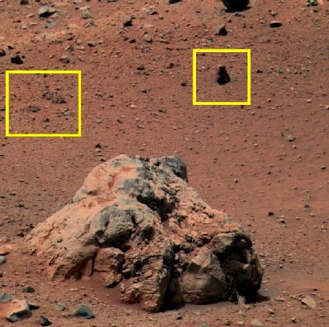
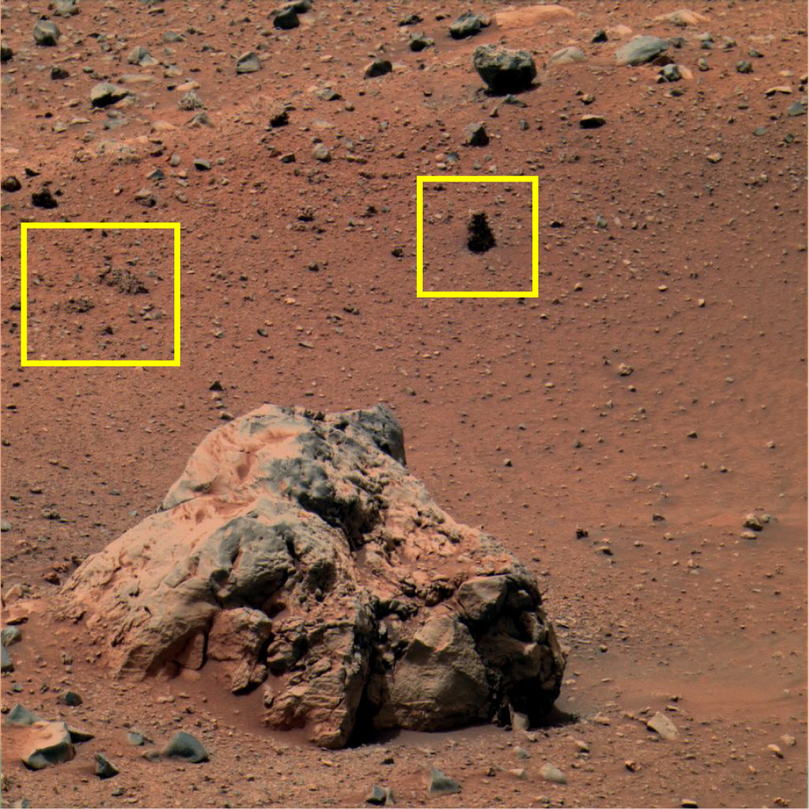
Wind direction on Mars
This image
from Spirit shows some nice evidence for the predominant wind
direction.
Yardangs on Mars. Wikipedia's page on Yardang
2-173059977-6.jpg - Some sort of drastic contact between rock/soil distributions.
Spirit has some nice vistas from the top of the hill out to Gusev's crater rim on the horizon.
Archaeologists figure out mystery of Stonehenge bluestones
Sun Ultra20 Opteron systems for $900 without going to eBay. Sounds like a way better machine than the 4 wimpy Sun Blade 100's that are running ~500MHz sparc ships, are slow, and have no firewire/usb2 ports for cheap and easy external drives.
Yardangs on Mars. Wikipedia's page on Yardang
2-173059977-6.jpg - Some sort of drastic contact between rock/soil distributions.
Spirit has some nice vistas from the top of the hill out to Gusev's crater rim on the horizon.
Archaeologists figure out mystery of Stonehenge bluestones
  ARCHAEOLOGISTS have solved one of the greatest mysteries of
  Stonehenge - the exact spot from where its huge stones were
  quarried.


  A team has pinpointed the precise place in Wales from where the
  bluestones were removed in about 2500 BC.


  It found the small crag-edged enclosure at one of the highest points
  of the 1,008ft high Carn Menyn mountain in Pembrokeshire's Preseli
  Hills.


  The enclosure is just over one acre in size but, according to team
  leader Professor Tim Darvill, it provides a veritable "Aladdin's
  Cave" of made-to-measure pillars for aspiring circle
  builders. Within and outside the enclosure are numerous prone pillar
  stones with clear signs of working. Some are fairly recent and a
  handful of drill holes attest to the technology used. Other blocks
  may have been wrenched from the ground or the crags in ancient
  times.


  They were then moved 240 miles to the famous site at Salisbury
  Plain, Wiltshire.
  ...
Sun Ultra20 Opteron systems for $900 without going to eBay. Sounds like a way better machine than the 4 wimpy Sun Blade 100's that are running ~500MHz sparc ships, are slow, and have no firewire/usb2 ports for cheap and easy external drives.
06.27.2005 06:17
Super easy multicast Twisted py example
Simple
UDP Multicast Client / Server using twisted
San Francisco Bay Area Tsunami map - do not try this from a dialup internet connection.
# Simple UDP Multicast Server example # Kyle Robertson # A Few Screws Loose, LLC # http://www.afslgames.com # ra1n@gmx.net # MulticastServer.pyTook me 2 minutes to try this and it worked right off. Nice!
from twisted.internet.protocol import DatagramProtocol from twisted.internet import reactor from twisted.application.internet import MulticastServer
class MulticastServerUDP(DatagramProtocol): def startProtocol(self): print 'Started Listening' # Join a specific multicast group, which is the IP we will respond to self.transport.joinGroup('224.0.0.1')
def datagramReceived(self, datagram, address): # The uniqueID check is to ensure we only service requests from ourselves if datagram == 'UniqueID': print "Server Received:" + repr(datagram) self.transport.write("data", address)
# Note that the join function is picky about having a unique object # on which to call join. To avoid using startProtocol, the following is # sufficient: #reactor.listenMulticast(8005, MulticastServerUDP()).join('224.0.0.1')
# Listen for multicast on 224.0.0.1:8005 reactor.listenMulticast(8005, MulticastServerUDP()) reactor.run()
#############################################################################
# Simple UDP Multicast Client example # Kyle Robertson # A Few Screws Loose, LLC # http://www.afslgames.com # ra1n@gmx.net # MulticastClient.py
from twisted.internet.protocol import DatagramProtocol from twisted.internet import reactor from twisted.application.internet import MulticastServer
class MulticastClientUDP(DatagramProtocol):
def datagramReceived(self, datagram, address): print "Received:" + repr(datagram)
# Send multicast on 224.0.0.1:8005, on our dynamically allocated port reactor.listenUDP(0, MulticastClientUDP()).write('UniqueID', ('224.0.0.1', 8005)) reactor.run()
San Francisco Bay Area Tsunami map - do not try this from a dialup internet connection.
06.26.2005 19:16
National Archives data volume issues
While waiting for my computer to
convert a massive postscript file to a tif, I ran into this very
interesting article on the issues faced by the National Archives
for the US Government:
feature memory
Comparison of broadband ISPs
... But saving the functionality of software--from desktop programs like Word to the software NASA used to test a virtual-reality model of the Mars Global Surveyor, for example--is a key research problem. And not all software keeps track of how it was actually used. Why might this matter? Consider the 1999 U.S. bombing of the Chinese embassy in Belgrade. U.S. officials blamed the error on outdated maps used in targeting. But how would a future historian probe a comparable matter--to check the official story, for example--when decision-making occurred in a digital context? Today's planners would open a map generated by GIS software, zoom in on a particular region, pan across to another site, run a calculation about the topography or other features, and make a targeting decision.What a great argument for open formats.
If a historian wanted to review these steps, he or she would need information on how the GIS map was used. But "currently there are no computer science tools that would allow you to reconstruct how computers were used in highconfidence decision-making scenarios," says Peter Bajcsy, a computer scientist at the University of Illinois at Urbana-Champaign. "You might or might not have the same hardware, okay, or the same version of the software in 10 or 20 years. But you would still like to know what data sets were viewed and processed, the methods used for processing, and what the decision was based on." That way, to stay with the Chinese embassy example, a future historian might be able to independently assess whether the database about the embassy was obsolete, or whether the fighter pilot who dropped the bomb had the right information before he took off. Producing such data is just a research proposal of Bajcsy's. NARA says that if such data is collected in the future, the agency will add it to the list of things needing preservation. ...
Comparison of broadband ISPs
06.26.2005 13:45
bash aliases for Adobe tools
The way I work on papers, I do a lot
from X11 xterms. I generate pictures with shell scripts (and
Fledermaus File->File->Screen Capture). Then I want to be
able to modify images with Adobe Photoshop and then composite the
image into a figure with Illustrator. I was getting frustrated
about having to go through the whole File->Open business, so I
created two little bash aliases in my ~/.bashrc file:
Just saw RayGUI in the March 2005 EOS. Sounds cool and it uses rayinvr which also sounds handy, but no available source? Then I am not really that interested. Why not just GPL this stuff? If it was GPL'ed, they could still sell it to companies for non-GPL'ed use. Or even use one of the more restrictive open source licenses. Having to email authors for source... then I can not put these two in fink.
alias photoshop='open -a /Applications/Adobe\ Photoshop\ CS/Adobe\ Photoshop\ CS.app'
alias illustrator='open -a /Applications/Adobe\ Illustrator\ CS/Illustrator\ CS.app'
Now I can just do things like this:
  photoshop capture1.png
  illustrator capture1-corrected.png
or
  photoshop capture0[2-5]*.png  # Open up capture02 to capture05!
Much easier!
Just saw RayGUI in the March 2005 EOS. Sounds cool and it uses rayinvr which also sounds handy, but no available source? Then I am not really that interested. Why not just GPL this stuff? If it was GPL'ed, they could still sell it to companies for non-GPL'ed use. Or even use one of the more restrictive open source licenses. Having to email authors for source... then I can not put these two in fink.
06.25.2005 08:32
Layback
Update: 28-Jun-2005
  The shot distance calculation method that uses the whole line is
  really not good.  As the water depth under the chirp changes, the
  time between pings (and hence distance between shots) changes.
One of the issues with chirp seismic profiles that I need to address is correlating the locations of cores to shot points that the chirp system records. This task is already handled for hull mounted systems, but must accounted for with towed systems like the one that Neal Driscoll has. Since the GPS is mounted on the ship and the fish is in the water on a cable, we need a way to know where the fish is relative to the the GPS. To make life easy, I am going to make some assumptions that are basically true for this cruise. Note that these assumptions are definitely not valid on other cruises.
- The ship is moving at a constant velocity
- The ship is moving in a straight line
- Nobody changed the wire out on the fish and the wire out is known
- The fish is stable in water column - not moving up and down
- The wire from the back of the ship to the fish is in a straight line. This is not totally true, but it should be close enough
- We have a large section of flat sea floor somewhere in the line
The first numbers come from the log book on page 9. The distance from the GPS antenna to the block right below the A-frame is 12 meters. The cable out from the block is 50m.
Next I need to get some depth points on a track line in an area near where the sea floor is basically flat. I used segysql.py to generate a database for bpsio04L04.xstar and created a lonlatshot log with this sqlite command:
  sqlite segy.db 'select x/3600.0,y/3600.0,Shotpoint from segyTrace'\
   | tr '|' ' '> lonlatshot.txt
Fledermaus is an easy way to get these values. I loaded the data object santabarbC_bath.sd which is the model for whole basin made by MBARI. Then File->Import->Import Line and use lonlatshot.txt as an xy data file. Then click the drape button to see the line right on the bathymetry. Zoom into the shelf edge where the line is. Put the mouse over a couple points on the line in a flat area:
  -120.05222321 34.40695572 -84.42
  -120.05193329 34.40694809 -84.28
I then went back into the lonlatshot.txt file and found that these points were are around shot 88450. I used pltsegy to show the shot range of 88200 to 88700. I then picked the sea floor and got this pick.xtp file:
88399    1     0.000   0.072
88451    1     0.000   0.071
88500    1     0.000   0.071
This means that the two way travel time (ttwt) between the fish and the sea floor is about 0.0714 seconds. If sound velocity in water is 1500 m/s, the two way time should be multiplied by 750 m/s to get distance.
0.0714 s * 750 m/s = 53.55m above the sea floor.We need the depth of the fish in the water to complete a right triangle: Water depth minus the distance above the sea floor.
84.3m - 53.55m = 30.75 meters below the surface.Then add 1 meter for the distance of the block above the sea surface. to get 31.75 meters. With 50 meters of wire out, we can now solve the equation x*x + y*y = wirelen*wirelen.
python -c "import math; print math.sqrt(50*50 - 31.75*31.75)"That 38.63 is the horizontal distance from the block to the fish. The total horizontal distance from the fish to the GPS needs to have the extra 12 meters of deck space added.
38.6256067914
38.63m + 12m = 50.63m behind the GPS.Now we need a simple shot offset: If we have a best fit match for a core to an xstar lon,lat,shot, How many shot points to add or subtract to where that core is by shot number in the chirp seismics? Since the fish is behind the ship, we have to add shots to the best fit shot to find the actual shot for that core location. How to figure the shot offset? We have to assume a constant speed and calculate an average distance per shot. We can use a whole straight line to figure this out. From lonlatshot.txt:
  -120.063888888889 34.3408333333333 79830
  -120.063888888889 34.3408333333333 79830
  ...
  -120.051388888889 34.4116666666667 89824
  -120.051388888889 34.4116666666667 89824
How far is that? We can use the proj USGS package with the UTM project to calculate distances in small areas like the Santa Barbara Basin. I talked about this in VizLecture 7. The Santa Barbara Basin is in UTM Zone 11S, but we just need the 11.
proj +proj=utm +zone=11Python can compute the distance in meters for us:
-120.063888888889 34.3408333333333 0. -120.051388888889 34.4116666666667 0.
Giving:
218142.35 3804201.63 0. 219529.19 3812025.38 0.
  python -c "import math; print math.sqrt( \
    pow(218142.35-219529.19,2)+pow(3804201.63-3812025.38,2)\
    )"


  7945.7151502
Now use that 7945.71 meters to get the meters/shot:
python -c "print 7945.72/(89824-79830)"So how many shots is 50.63 meters?
0.795049029418 meters/shot
python -c "print 50.63/0.79505"A little bash script will help make a table of the core locations and best fit.:
63.6815294636 Shots
for file in ?-find.dat; do echo -n "$file: ";head -8 $file | tail -1 doneNow for the best matching shot number with layback:
1-find.dat: -120.108056 34.361111 0.000079 48 245237 4041 2-find.dat: -120.107778 34.369722 0.000393 48 245985 5537 3-find.dat: -120.058889 34.365556 0.000124 17 81682 3727 4-find.dat: -120.057222 34.378889 0.000124 17 83033 6424 5-find.dat: -120.023611 34.336667 0.000386 57 293301 15245 6-find.dat: -119.977222 34.328333 0.001650 58 296308 1255
(for file in ?-find.dat; do echo -n "$file: ";head -8 $file |\
 tail -1 ; done) | awk '{print $1,$6+64}'


1-find.dat: 245301
2-find.dat: 246049
3-find.dat: 81746
4-find.dat: 83097
5-find.dat: 293365
6-find.dat: 296372
And that is the table of the best shot for each core!There are several other ways to calculate the layback and most of them are better than this one! Jenna used a method that uses an area of the chirp where the water multiple is visible in the sampling window. This gives water depth. Using this method is would be possible to build a lookup table of speed to depth.
An even better solution is to have a depth transducer on the fish and an encoder on the winch. Then use a more complete wire/flight model for the fish.
Thanks to R. Fenwick and J. Hill for help on this.
Fashion of the day in PB: "Utilikilts"
06.25.2005 07:56
Firefox security hole
Nice web page Jeff: Jeff Sorrentino. I like the
photo map of Japan.
Just read a little article on lwn.net about a Firefox features that is really scary. I can think up quite a few ways to abuse this in just a couple minutes, especially by putting this kind of thing in comments to popular websites.
Just read a little article on lwn.net about a Firefox features that is really scary. I can think up quite a few ways to abuse this in just a couple minutes, especially by putting this kind of thing in comments to popular websites.
  <link rel="prefetch" href="URL">


  Google's use of prefetching in this way is unfortunate; it seems
  certain to lead to trouble for somebody, somewhere down the
  line. The real problem, however, is with Firefox, which is shipped
  with prefetching turned on. There is no indication, anywhere in the
  preference screens, that an option controlling prefetching even
  exists. Anybody wanting to disable prefetching will have to edit
  their prefs.js file, or tweak the network.prefetch-next option on
  the about:config screen. Turning off prefetch in this way will slow
  down some page loads, but, for many users, the extra delay will be
  worth it.
06.24.2005 20:03
Release the hostage!
So I just got a very strange phone
call:
Me:        "Hello"
Some lady: "When are you going to release the hostage?"
Me:        "Excuse me?"
Lady:      "When are you going to release the hostage?"
Me:        "What?"
Lady:      "My jacket!"
Me:        "Who is this?"
Lady:      "Sorry."    *** Click. ***
That was different.
06.24.2005 08:42
segy-py 0.14, now with makepltsegy.py
Segy-py version 0.14 is
out. I added a script to generate sample pltsegy input files. Also
the gmt datafile generation now does the right thing with fileKey
ranges. If you do not specify a range, it uses all the files.
Top 10 Cell Phone Wish List. My favorites:
Top 10 Cell Phone Wish List. My favorites:
- One standard connector for power for all phones. I know that means they will sell fewer power adaptors.
- Put a USB port on the thing and let us use it all! Why do I have to send my pictures????
- Allow Data Backups on Carrier Servers
06.23.2005 21:35
Dibblee maps California, Mac OSX backups, OSX tips
  Dibblee, T.W. (1982). Regional Geology of the Transverse Ranges
  Province of southern California. In: Geology and Mineral Wealth of
  the California Transverse Ranges., edited by Fife, D. L., and Minch,
  J. A. South Coast Geological Society, Annual Symposium and Guidebook
  10, 7-26
How did Dibblee publish all of those papers and maps on California geology? I ran into this reference today and had flash backs to my undergrad with Stanford Geology field trips. Dibblee would always have something relevant to where ever we went. Did he map from a race car or something?
Just saw a great Mac OSX tip:
Multi-DVD or (multi-CD) spanning backups with tar. This tip uses xtar with the -m flag for multivolume support. Now that I look at the standard GNU tar on OSX, I see that it has the option --multi-volume that I had never noticed before. Very interesting. What happens if I loose, say, the middle CD of 3? Can I still get the rest back? What about files that are larger than 1 CD? What happens then?
Many Mac OSX tips. I like many of these. Especially cool are:
[For bash, just] put this in your ~/.inputrc file:
  set completion-ignore-case On


Converting from DOS to unix line terminators (Unix->General)
   perl -pi -e 's/ / /g' mealcsv.csv


ind . -name "*.h" -exec grep NSDoWhatIMean {} ; -print


hdiutil mount diskimage.dmg


Seeing the console.log without running Console.app (Unix->General)
In a terminal or an emacs shell:
% tail -f /var/tmp/console.log


Media types supported
  drutil info


Building projects from the command line (Project Builder->General)
  Look at pbxbuild


Core files seem to be getting dumped into /cores, rather than the
directory the program was run from


Showing current column position (emacs->General)
  M-x column-number-mode


Turning off incremental-search highlighting (emacs->General)
Emacs 21, which comes with Mac OS X 10.2, has highlighting enabled when doing incremental search (which drives me nuts). You can turn that off by setting this in your .emacs file:
(setq search-highlight nil)


You may also need to
(setq isearch-lazy-highlight nil)


Running a screensaver as your desktop background (Screen Savers->Random)
In a terminal, run
% /System/Library/Frameworks/ScreenSaver.framework/Resources/ScreenSaverEngine.app/Contents/MacOS/ScreenSaverEngine -background &
Wow... I am not even half way through that file. I especially like that last one.
06.23.2005 18:15
more links
JavaScript Toolbox. e.g.
Uses DHTML to turn an ordinary
list into a dynamic, expandable,
collapsable tree structure. No javascript coding required! VisCheck simulates colorblind
vision.
I am amused to think that ad blocking systems in web browsers would mark an end to content. I seem to remember quite of few very exciting web pages in the days before DoubleClick/BetterClick/Google AdSense. I am sure that DoubleClick will work hard to thwart Adblock.
I am amused to think that ad blocking systems in web browsers would mark an end to content. I seem to remember quite of few very exciting web pages in the days before DoubleClick/BetterClick/Google AdSense. I am sure that DoubleClick will work hard to thwart Adblock.
06.23.2005 13:47
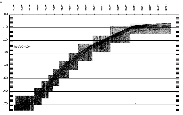
sioseis and pltsegy continued
My seismic lines that I have been
working on is starting to look much better. The biggest
improvements have come with doing a better job of picking the water
bottom. The first trick is to really expand sections of the line
and pick those. The screen resolution is a real limiting factor.
With Becca's help, I have turned on filtering and trace mixing within sioseis. My procs line now looks like this:
Almost forgot. Here is the current command line for the sioseis script.
        shb = 81800; { beginning shot
        shf = 82800; { ending shot
        timscal= 300; { suggest 1000 to 200 for chirp
        tmark = 0.09; { get the horizontal lines out of the way.
        spa = 0.2;    { horzontal spacing
First, only plot a thousand shots at a time. Then jack up the
timscal to increase the vertical size. The spa up to take up more
of the screen horizontally.With Becca's help, I have turned on filtering and trace mixing within sioseis. My procs line now looks like this:
procs diskin header filter wbt mix gains prout diskoa enwith the addition of the filter and mix sections. I did not totally understand the mix web page, so it was great to have an example to copy.
filter fno $FNO lno $LNO ftype 99 pass 150 6500 end endThe final trick really is to write out postscript which is then converted to tif by ghostscript (gs).
mix fno $FNO lno $LNO type 1 weight 0.25 0.50 0.25 end end
Almost forgot. Here is the current command line for the sioseis script.
./sioseis-wbt.bash bpsio04L04.sgy bpsio04L04-wbt04.sgy \
bpsio04L04-04.h2o bpsio04L04-02.gains
Now all I need is layback to figure out where the cores really
should be.06.22.2005 19:28
Using segysqldist and pltsegy
Now I am actually working on data
that I know is of use to my thesis. I need to make the plot look
'reel purdy' this evening. Here are some notes on how I am doing
this.
I am starting with the same xstar file that I was working with yesterday: bpsio04L04.xstar. It would be nice to have a little option that would calculate the bounding box for a line, but I do not have that at the moment. What I do have is segysqldist.py. First I need a database just for this line (so it will go quickly).
Now I just have to look in the results-lonlat.dat file to find out which shots to work with in pltsegy.
I am starting with the same xstar file that I was working with yesterday: bpsio04L04.xstar. It would be nice to have a little option that would calculate the bounding box for a line, but I do not have that at the moment. What I do have is segysqldist.py. First I need a database just for this line (so it will go quickly).
> segysql.py -f bpsio04L04.db -d xstar bpsio04L04.xstar
> ls -l bpsio04L04.db
-rw-r--r-- 1 schwehr staff 27310080 Jun 22 19:18 bpsio04L04.db
Now I would like to see how this line compares to the core 4
location. My new app segysqldist.py is designed just for this job.
> segysqldist.py -x -120.05716666 -y 34.37899999 -n 100 \
-d line.dat -f bpsio04L04.db
Starting SQL select. This make take quite a while
Finished SQL select
# Beginning search
Using slower search for many points. Suggest using -n 1 for faster
Inspecting data:
1000
2000
...
> ls -ltr | tail -4
-rw-r--r-- 1 schwehr staff 168 Jun 22 19:26 coreloc.dat
-rw-r--r-- 1 schwehr staff 21 Jun 22 19:32 point.dat
-rw-r--r-- 1 schwehr staff 3500 Jun 22 19:32 results-lonlat.dat
-rw-r--r-- 1 schwehr staff 552863 Jun 22 19:32 line.dat
The program created 3 new files. point.dat contains the location
that was specified on the command line to search for.
results-lonlat.dat has the closest 100 shots (ignoring all the
shots with duplicate locations). Finally line.dat has a subsampled
set of x,y pairs of the input data so that we can see the track
lines. Now I need to use my trusty friend gnuplot to see what the
world looks like.
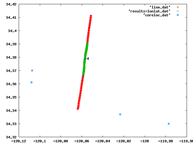
gnuplot> plot 'line.dat','results-lonlat.dat','coreloc.dat' gnuplot> set label 4 '4' at -120.055,34.37899999 gnuplot> set terminal png gnuplot> set output '4-distance.png' gnuplot> plot 'line.dat','results-lonlat.dat','coreloc.dat'In the graph, the green section (I know... red/green = bad) marks the closest 100 shot locations that surround core 4.
Now I just have to look in the results-lonlat.dat file to find out which shots to work with in pltsegy.
> head -15 results-lonlat.dat # segysqldist.py # # distance - currently is in "degrees"... sort of # traceNumber - the offset in the particular segy file # fileKey - use the segyFile table in *.db to translate # # longitude latitude "distance" fileKey Shotpoint traceNumber -120.057222 34.378889 0.000124 1 83033 6424 -120.056944 34.378889 0.000248 1 83059 6476 -120.056944 34.379167 0.000278 1 83069 6496 -120.057222 34.378611 0.000393 1 82994 6346 -120.056944 34.379444 0.000497 1 83106 6570 -120.057222 34.378333 0.000669 1 82956 6270 -120.056944 34.379722 0.000756 1 83143 6645 -120.057222 34.378056 0.000946 1 82922 6202There is a handy program called minmax in GMT that will summarize the situation for us!
> minmax results-lonlat.datThis means that the key range in pltsegy is in the neighborhood of shotpoints 81820 to 84782. I am going to round this to be a nicer range for plotting in pltsegy.
results-lonlat.dat: N = 100 <-120.059/-120.055> <34.3672/34.3908> <0.000124/0.012083> <1/1> <81820/84782> <4001/9921>
81800 to 84800Hopefully my makepltsegy.py script will actually work to give a plot in this range. I need to adjust sioseis-wbt.bash to only spit out this region for the maximum turnaround time.
declare -r FNO="81800" declare -r LNO="84800" declare -r INFILE=$1 declare -r OUTFILE=$2 declare -r WBTFILE=$3And run sioseis something like this:
> ./sioseis-wbt.bash bpsio04L04.sgy bpsio04L04-wbt03.sgy \
bpsio04L04-02.h2o
> ls -l *.sgy
-rwxr-xr-x 1 schwehr staff 81956368 Jun 21 11:31 bpsio04L04-wbt01.sgy
-rwxr-xr-x 1 schwehr staff 81956368 Jun 21 21:04 bpsio04L04-wbt02.sgy
-rwxr-xr-x 1 schwehr staff 24890896 Jun 22 20:20 bpsio04L04-wbt03.sgy
This gives a much smaller (24MB) seismic file to work with in the
short term. Off to constructing the pltsegy file. Ouch... I am
getting a slightly frustrating error:
> rm -f sort*; pltsegy test.pltsegy ***NMLST error. Supplied name doesnt appear in table Error was in timescal = reduc -2.58253e-29 *** Error (PLOTS). Invalid device number = -1073744224 Valid devices are:- Landscape: device 16 Portrait: device 17 (Default)X Landscape: device -1 Postscript Portrait: device 14 Postscript Landscape: device 15I am not sure what that means. My previous pltsegy file still works fine and is not too different. Would help if I knew what kind of parser is in pltsegy, but I am not motivated enough to go look. Here is the beginning of the offending file:
plot
dtfile = bpsio04L04-wbt03.sgy;
plfile = test.ps;
srtfile = sort.test.pltsegy.sort;
cdp = t;
device = 16;
interact = 1;
size = 550, 350;
sort = shot;
shb = 81800; { beginning shot
shf = 84800; { ending shot
noinc = 1;
ntrab = 1;
ntraf = 1;
ntrinc = 1;
speq = t;
delt = 0.000083;
tbi = 0.0;
tfi = 0.75;
timescal = 200;
tmark = 0.01;
spa = 0.025;
...
Oh... typo! Should be timscal, not timescal. Got it. Now I
have a happy pltsegy. To make the plot take up more of the
horizontal screen space I had to adjust the horizontal shot spacing
(spa).
> makepltsegy.py -o test.pltsegy -p test.ps -i bpsio04L04-wbt03.sgy \
-s 81800 -S 84800 --spa=0.100 --timscal=200
> rm -f sort*; pltsegy test.pltsegy
Works!06.22.2005 19:15
link-a-lony
Open
source web design. We'll see what Susie, and Scott S. have to
say about these. Anyone want to say if this code is good? I noticed
that the front page is not rendering right on Safari 1.3 (Mac OSX
10.3.9) - Whoops!
I have never used ebay, but these tips are probably a little basic.
Panda 3D is a python system for 3D from CMU (now) and formerly from Disney.
More Schematics - like I have time to build anything right now!
PlotIP says that I am at 32.71528° N, 117.15639° W right now.
Errr. Bailey stole my chair after dinner, so I am now sitting on a small coffee table to use my computer on the card table. Fancy digs. Now I am starting to tweak gains. Woo hoo.
06.22.2005 10:57
segy-py 0.13 released
Segy-py release 0.13 adds
the segysqldist.py command line application. This uses the SQL
database to find the closest points to a target location. The
program needs a little more work, but it is basically working. Just
stay in small areas right now as the distance calculation is total
hack.
06.22.2005 07:50
closest shot to a lon,lat position
Patent
absurdity by Richard Stallman. If you think software patents
are good, you should read this article.
Becca and I talked some more yesterday about seismic data processing. There are big issues with surfaces with big slopes. Even small errors can produce huge errors. We really need a way to calculate layer thickness that is perpendicular to bedding. On steep slopes, a bed of zero thickness can get contorted to a rapidly changing bed up to meters thick which which know is no there at all.
When working with this stuff, "Gnuplot is the bomb!" We were quickly able to see what our picks look like. The 750 below converts to meters from time. Here is an example from memory.
I needed a quick algorithm to calculate distance between to locations on the Earth's geoid (I don't want to know about height). Wikipedia came through with great circle distance complete with a test case. This is not the best method for points close together but it works. What I really need is a python wrapper for Proj.4 (the USGS projection library). I think the gdal package as a pretty complete python interface to coordinate frame conversions, but the fink build explicitly excludes the python interface. Doh!
The new application that I am working on is called "segysqldist.py." It uses an SQL database of the trace header data to speed up the search. Right now, I am just using two lines. My next task is to have the program be able to find the N closest points so I can plot up the location and shots to see how they relate. The cores from last years cruise were taken on crossing lines or very close to crossing points. Location animated gif
On pltsegy: I was getting annoyed by the jagged, upside-down staircase underneath my plots with pltsegy. Becca pointed out that the gains set in sioseis can be used to get rid of most of them. Just drop the gain down a ways after a you think there will be no more good data (just noise and multiples). Dangerous, but works great.
Some interesting features seen by Spirit. Weathered rocks or something else?
Becca and I talked some more yesterday about seismic data processing. There are big issues with surfaces with big slopes. Even small errors can produce huge errors. We really need a way to calculate layer thickness that is perpendicular to bedding. On steep slopes, a bed of zero thickness can get contorted to a rapidly changing bed up to meters thick which which know is no there at all.
When working with this stuff, "Gnuplot is the bomb!" We were quickly able to see what our picks look like. The 750 below converts to meters from time. Here is an example from memory.
gnuplot
f(x) = 750 * x
plot 'top.h2o' using 1:(f($2)) with lp,\
'bot.h2o' using 1:(f($2)) with lp
set terminal pdf
set output 'layer-picks.pdf'
replot
quit
open layer-picks.pdf
My project that I started working on yesterday is to create a
python program that can find the closest shots to a point. I want
to know what file, shotpoint, and tracenum (the offset in the segy
file for the shot) that best shows a particular core.I needed a quick algorithm to calculate distance between to locations on the Earth's geoid (I don't want to know about height). Wikipedia came through with great circle distance complete with a test case. This is not the best method for points close together but it works. What I really need is a python wrapper for Proj.4 (the USGS projection library). I think the gdal package as a pretty complete python interface to coordinate frame conversions, but the fink build explicitly excludes the python interface. Doh!
The new application that I am working on is called "segysqldist.py." It uses an SQL database of the trace header data to speed up the search. Right now, I am just using two lines. My next task is to have the program be able to find the N closest points so I can plot up the location and shots to see how they relate. The cores from last years cruise were taken on crossing lines or very close to crossing points. Location animated gif
On pltsegy: I was getting annoyed by the jagged, upside-down staircase underneath my plots with pltsegy. Becca pointed out that the gains set in sioseis can be used to get rid of most of them. Just drop the gain down a ways after a you think there will be no more good data (just noise and multiples). Dangerous, but works great.
Some interesting features seen by Spirit. Weathered rocks or something else?
06.21.2005 15:46
More pltsegy
I have been working a little more
with pltsegy. Now is when I really could use a G5 machine. My lab
book makes a nice prop for the laptop to help it cool. I also
turned the window fan on me and the laptop. Ouch it gets hot!
Becca says that I need to say a bit more about picking the water bottom/sediment interface... When you run pltsegy with "device=16", it displays the seismic line on the screen (in an X11 window). You can click with the mouse on the sed/water interface (or any layer that you are trying to map) and a small 'x' will appear. Do this across the whole surface. When you have finished this, press the "dump" button on the left and look in the window. There will be some numbers that are also in the "pick.xtp" file. The 1st column is the shotpoint and the 4th column is the time of the pick (time 0 is the chirp fish in the water). Then you can use the awk script to make this a wbt input for sioseis. I just altered the sioseis script to allow you to specify the wbt as an input file. This will make things a little more scriptable with less emacs time. I still need to make the shot range be selectable from the command line. The new script gets run like this:
Becca says that I need to say a bit more about picking the water bottom/sediment interface... When you run pltsegy with "device=16", it displays the seismic line on the screen (in an X11 window). You can click with the mouse on the sed/water interface (or any layer that you are trying to map) and a small 'x' will appear. Do this across the whole surface. When you have finished this, press the "dump" button on the left and look in the window. There will be some numbers that are also in the "pick.xtp" file. The 1st column is the shotpoint and the 4th column is the time of the pick (time 0 is the chirp fish in the water). Then you can use the awk script to make this a wbt input for sioseis. I just altered the sioseis script to allow you to specify the wbt as an input file. This will make things a little more scriptable with less emacs time. I still need to make the shot range be selectable from the command line. The new script gets run like this:
./sioseis-wbt.bash bpsio04L04.sgy bpsio04L04-wbt02.sgy bpsio04L04-02.h2oHere is the script. I have marked the `cat $WBTFILE` line in black, which is the key change (in addition to the command line arg checking/handling).
#!/bin/bashThe next task to try out is writing to postscript with pltsegy. Postscript output will look a lot better than what you can do with just the screen. The trick is to change the device in the pltsegy device from 16 to 15. Remember that '{' is the comment character!
# First try at wbt declare -ri EXIT_FAILURE=1
if [ $# != 3 ] ; then echo echo " ERROR: Must specify 3 arguments. Found $#" echo echo " usage: $0 [segy in file] [segy out file] [wbt-pick-file] " echo echo " Example:" echo " $0 basic.sgy basic-wbt.sgy basic-picks.h2o" exit $EXIT_FAILURE fi
declare -r FNO="80000" declare -r LNO="89800" declare -r INFILE=$1 declare -r OUTFILE=$2 declare -r WBTFILE=$3
# FIX: allow user to specify FNO and LNO #procs diskin wbt gains header prout diskoa end
#cat << eof1 sioseis << EOF procs diskin wbt gains header prout diskoa end diskin ipath $INFILE end end
header fno $FNO lno $LNO l6 = l3 end end
wbt `cat $WBTFILE` end
wbt2 solrat 1.5 ses 0.049 0.05 sel 0.017 0.025 track 0.0005 end end
wbt3 thres 0.000000005 track 0.005 end end
filter
 fno $FNO lno $LNO ftype 99  pass 150 6500 end
end


mix
 fno $FNO lno $LNO type 1 weight 0.25 0.50 0.25 end
end
agc fno $FNO lno $LNO winlen .005 pctagc 90 end end
gains fno $FNO lno $LNO addwb yes type 9 TGP 0.0000 01.0000 0.0001 05.0000 0.0100 10.0000 0.0200 40.0000 0.0300 50.0000 0.0350 60.0000 0.0400 55.0000 0.0500 40.0000 end end
prout fno $FNO lno $LNO ftr 0 ltr 1 noinc 100 end end
diskoa opath $OUTFILE fno $FNO lno $LNO ftr 0 ltr 1 end end
end EOF
       {device = 16; { X11 screen
       device = 15; { postscript
Run pltsegy and wait a while until it finishes.
> ls -l *.ps
-rw-r--r--    1 schwehr  staff    101188928 Jun 21 15:27 bpsio04L04-wbt02.ps
Now use ghostscript to create a tif file from the postscript file. This will take a long time. Make sure your computer has proper cooling!
  > gs -sDEVICE=tiff24nc -r300 -sOutputFile=bpsio04L04-wbt02.tif bpsio04L04-wbt02.ps
  convert bpsio04L04-wbt02.tif bpsio04L04-wbt02.png
I am now trying to play with the shad argument.
- -1 gives all black
- 0 gives all black
- 1 gives all black
- 2 gives all white
- 3 gives nothing
- 5 gives the usual reasonable plot
06.21.2005 15:05
red tide sat photos
Satellite observations of the Southern California - "red tide"
by Mati Kahru.
Apple News: Apple Drops Single Processor Power Macs. Wow! Only dual processor machines for the deskside machines. Hopefully the prices come down too.
From the the Mom news service:
Portsmouth map
From Oar House History:

Apple News: Apple Drops Single Processor Power Macs. Wow! Only dual processor machines for the deskside machines. Hopefully the prices come down too.
From the the Mom news service:
Portsmouth map
From Oar House History:
06.21.2005 14:19
GIS city data
From Scripps:
Unlimited free hosting for your files - sounds nice. Maybe that is where I should put my big data files from my web server.
For MS windows: ccleaner.com. Is this any good/safe????
Google sight seeing update. Includes Iceland. Hey Google: How about Porthsmouth?
Electronic Schematics for Hobbyists
  Once again I have the sad duty to inform you of the passing of a
  respected and loved member of the Scripps community.  Dave Keeling
  died Monday evening of a sudden and unexpected heart attack,
  following a short hike in his beloved Montana.
From the slashdot department: Court Rules GIS Data Can't Be Kept Secret. City must release electronic GIS mapping data
  Silverbear writes "In an update from a Slashdot story posted in
  January, The Connecticut Supreme Court has ruled that there is not a
  significant security risk to the town of Greenwich in making its GIS
  Data available to the public, and therefore must do so. Greenwich
  had claimed that the data could compromise personal and national
  security, and was sued under CT Freedom of Information laws. The
  legal ruling is available."
Python: Evaluate using Decimals instead of floats.
Unlimited free hosting for your files - sounds nice. Maybe that is where I should put my big data files from my web server.
For MS windows: ccleaner.com. Is this any good/safe????
Google sight seeing update. Includes Iceland. Hey Google: How about Porthsmouth?
Electronic Schematics for Hobbyists
06.21.2005 09:36
sioseis and pltsegy
Now I am going to try to work through
a seismic line on my own without anyone arround to baby site and
without internet. This will be the true test
But first, what does it mean when a CA license plate has "LIVERY" at the bottom?
For this all to work, you must have segydump.py, sioseis, and pltsegy all in your path. Here is my particular setup.
Setup phase. The Babcock/Kent/Dingler convention for script files is to have them start with C_, which I think means "command."
Looking at the file size for the xstar and sioseis segy files, you will see that the sgy is about 1/2 the size of the xstar. This is because sioseis turns the "complex" two trace values from xstar into a "real" value (I think using a Hilbert transform).
Another thing to note is that in the header field above, I used "fno 0 lno 999999 ftr 0 ltr 999999". This is an attempt to write all of the traces.
Now I need to know the beginning and end shot numbers for the file. I will show two ways to do this: first with segydump.py and second with sutil.
Now I know that the shots in this file go from 79818 to 89824. Now I can move on to using pltsegy to give a first view of the data. I have to use pltsegy files from templates or I am lost. I will start with one from Becca and go from there. I will just paste it in. This will be long! Plt_ice2001L28
But first, what does it mean when a CA license plate has "LIVERY" at the bottom?
For this all to work, you must have segydump.py, sioseis, and pltsegy all in your path. Here is my particular setup.
> sioseis
  SIOSEIS ver 2005.1 (7 Feb. 2005)  (C) Regents of U.C.
> segydump.py --version
  segydump.py 0.13 - 1.11


> type -a  pltsegy pltsegy_prep.macX sioseis segydump.py
pltsegy is /Users/schwehr/bin/pltsegy
pltsegy_prep.macX is /Users/schwehr/bin/pltsegy_prep.macX
sioseis is /Users/schwehr/bin/sioseis
segydump.py is /Users/schwehr/x/src/segy-py/segydump.py
Setup phase. The Babcock/Kent/Dingler convention for script files is to have them start with C_, which I think means "command."
   cd ~/Desktop/Segy/
   mkdir Try2         # Try1 was coached by Becca... thanks Becca!
   cp xstar/bpsio04L04.xstar.bz2 Try2/
   cp DinglerClassNotes/C_ConvertXstar_CMT Try2
The real the first step was to pull the data off of the cruise tapes using my readtape.bash script, but I did that last year. The resulting xstar files are in the EdgeTech XSTAR format which most seismic systems have trouble with. Paul Henkart has written a special "format edgetech" to pull in these files. I will first use sioseis to convert xstar to a sioseis sgy file. I rewrote Jeff D.'s script to be xstar2segy.bash. This has only the sioseis conversion script.
#!/bin/bashNow to run the script:
declare -ri EXIT_FAILURE=1
if [ $# != 2 ] ; then echo "usage: [Input XstarFile] [Output SegyFile] " ; exit $EXIT_FAILURE fi
#################################### # Convert Xstar to Segy. Must use 10Aug2004 version of SIOSEIS or newer # course and speed located in i63 & i64
# xstar variable dummies is a switch indicating how the program should treat # missing pings or a missing ducer on the dual ducer xstar. When dummies = 2, # when 1 ducer is missing, the single trace is scaled and output. Missing pings # are replaced by dead traces.
sioseis << EOF procs diskin xstar header diskoa end
diskin format edgetech ipath $1 end end
xstar type 2 dummies 2 end end
header fno 0 lno 999999 ftr 0 ltr 999999 l3 = l1 l6 = l3 end end
diskoa opath $2 end end
end EOF echo "Done."
./xstar2segy.bash bpsio04L04.xstar bpsio04L04.sgy
  SIOSEIS ver 2005.1 (7 Feb. 2005)  (C) Regents of U.C.
 procs diskin xstar header diskoa end

 diskin
     format edgetech
     ipath bpsio04L04.xstar end
 end
  ...


 diskoa
   opath bpsio04L04.sgy end
 end

 end
 ****    0 ERRORS IN THIS JOB   ****
  Ping has only 1 ducer.
  Ping has only 1 ducer.
  ...
  Ping has only 1 ducer.
  Ping has only 1 ducer.
  Ping has only 1 ducer.
 1 missing pings will be replaced by dead ones.
  Ping has only 1 ducer.
  Ping has only 1 ducer.
  Ping has only 1 ducer.
  ...
  Ping has only 1 ducer.
 1 missing pings will be replaced by dead ones.
  END OF SIOSEIS RUN
Done.


> ls -l bp*
-rwxr-xr-x    1 schwehr  staff    83652112 Jun 21 10:04 bpsio04L04.sgy
-rwxr-xr-x    1 schwehr  staff    163843600 Jun 21 09:39 bpsio04L04.xstar


> md5 bp*
MD5 (bpsio04L04.sgy) = 8f4bd9e3bf622efa59176ce020369c76
MD5 (bpsio04L04.xstar) = 2ddcb3f76d1df7ee21da69d3aa568b60
Keeping a record of md5 sums for seismic files is not a bad idea.
Then you can know for sure if you are working with the exact same
file at a later date. This can be critical if there has been a
change in, for example, the way that sioseis handles xstar data or
a change with the header reassignments (e.g. l3=l1 l6=l3).Looking at the file size for the xstar and sioseis segy files, you will see that the sgy is about 1/2 the size of the xstar. This is because sioseis turns the "complex" two trace values from xstar into a "real" value (I think using a Hilbert transform).
Another thing to note is that in the header field above, I used "fno 0 lno 999999 ftr 0 ltr 999999". This is an attempt to write all of the traces.
Now I need to know the beginning and end shot numbers for the file. I will show two ways to do this: first with segydump.py and second with sutil.
> segydump.py -d xstar -t 1 bpsio04L04.xstar | grep ShotpointMake sure that you specify the xstar driver or you will get crazy results when using segydump.py.
1: LineSeqNo=79818
> segydump.py -d xstar -t -1 bpsio04L04.xstar | grep Shotpoint
20000: LineSeqNo=89824
==============================
> sutil Enter SEG-Y file name: bpsio04L04.sgy
OVERVIEW: Data format: IEEE floating point Total # of traces: 10211 dt (milliseconds): 0.083 samples/trace: 1988
shot (trc) cdp (trc) 0ffset ======================================================================== First trc: 79818 1 79818 0 0 Last trc: 89824 1 89824 0 0 ========================================================================
Now I know that the shots in this file go from 79818 to 89824. Now I can move on to using pltsegy to give a first view of the data. I have to use pltsegy files from templates or I am lost. I will start with one from Becca and go from there. I will just paste it in. This will be long! Plt_ice2001L28
plot
       dtfile = ice2001L28.P.sgy;
       plfile = ice2001L28.ps;
       srtfile = sort.ice;
       cdp = t;
       device = 16;
       interact = 1;
       size = 550, 350;
       sort = shot;
       shb= 116000;
       shf = 130000;
       noinc = 1;
       ntrab = 1;
       ntraf = 1;
       ntrinc = 1;
       speq = t;
       delt = 0.000083;
       tbi = 0.05;
       tfi = 0.25;
       timscal = 1000;
       tmark = 0.01;
       spa = 0.025;
       negpol= f;
       form = I6;
       anninc = 500;
       xann = 116000;
       delann = 1;
       reduc = 1.00;
       clip = 1.0;
       {mxdef = -1.0;
       pscale = 30000000;
       rtl = f;
       shad = 5;
       level =
     0.007874
     0.015748
     0.023622
     0.031496
      0.03937
     0.047244
     0.055118
     0.062992
     0.070866
      0.07874
     0.086614
     0.094488
      0.10236
      0.11024
      0.11811
      0.12598
      0.13386
      0.14173
      0.14961
      0.15748
      0.16535
      0.17323
       0.1811
      0.18898
      0.19685
      0.20472
       0.2126
      0.22047
      0.22835
      0.23622
      0.24409
      0.25197
      0.25984
      0.26772
      0.27559
      0.28346
      0.29134
      0.29921
      0.30709
      0.31496
      0.32283
      0.33071
      0.33858
      0.34646
      0.35433
       0.3622
      0.37008
      0.37795
      0.38583
       0.3937
      0.40157
      0.40945
      0.41732
       0.4252
      0.43307
      0.44094
      0.44882
      0.45669
      0.46457
      0.47244
      0.48031
      0.48819
      0.49606
      0.50394
      0.51181
      0.51969
      0.52756
      0.53543
      0.54331
      0.55118
      0.55906
      0.56693
       0.5748
      0.58268
      0.59055
      0.59843
       0.6063
      0.61417
      0.62205
      0.62992
       0.6378
      0.64567
      0.65354
      0.66142
      0.66929
      0.67717
      0.68504
      0.69291
      0.70079
      0.70866
      0.71654
      0.72441
      0.73228
      0.74016
      0.74803
      0.75591
      0.76378
      0.77165
      0.77953
       0.7874
      0.79528
      0.80315
      0.81102
       0.8189
      0.82677
      0.83465
      0.84252
      0.85039
      0.85827
      0.86614
      0.87402
      0.88189
      0.88976
      0.89764
      0.90551
      0.91339
      0.92126
      0.92913
      0.93701
      0.94488
      0.95276
      0.96063
       0.9685
      0.97638
      0.98425
      0.99213
            1;
       palette =
  255.0000  255.0000  255.0000
  253.0078  253.0078  253.0078
  251.0156  251.0156  251.0156
  249.0234  249.0234  249.0234
  247.0312  247.0312  247.0312
  245.0391  245.0391  245.0391
  243.0469  243.0469  243.0469
  241.0547  241.0547  241.0547
  239.0625  239.0625  239.0625
  237.0703  237.0703  237.0703
  235.0781  235.0781  235.0781
  233.0859  233.0859  233.0859
  231.0938  231.0938  231.0938
  229.1016  229.1016  229.1016
  227.1094  227.1094  227.1094
  225.1172  225.1172  225.1172
  223.1250  223.1250  223.1250
  221.1328  221.1328  221.1328
  219.1406  219.1406  219.1406
  217.1484  217.1484  217.1484
  215.1562  215.1562  215.1562
  213.1641  213.1641  213.1641
  211.1719  211.1719  211.1719
  209.1797  209.1797  209.1797
  207.1875  207.1875  207.1875
  205.1953  205.1953  205.1953
  203.2031  203.2031  203.2031
  201.2109  201.2109  201.2109
  199.2188  199.2188  199.2188
  197.2266  197.2266  197.2266
  195.2344  195.2344  195.2344
  193.2422  193.2422  193.2422
  191.2500  191.2500  191.2500
  189.2578  189.2578  189.2578
  187.2656  187.2656  187.2656
  185.2734  185.2734  185.2734
  183.2812  183.2812  183.2812
  181.2891  181.2891  181.2891
  179.2969  179.2969  179.2969
  177.3047  177.3047  177.3047
  175.3125  175.3125  175.3125
  173.3203  173.3203  173.3203
  171.3281  171.3281  171.3281
  169.3359  169.3359  169.3359
  167.3438  167.3438  167.3438
  165.3516  165.3516  165.3516
  163.3594  163.3594  163.3594
  161.3672  161.3672  161.3672
  159.3750  159.3750  159.3750
  157.3828  157.3828  157.3828
  155.3906  155.3906  155.3906
  153.3984  153.3984  153.3984
  151.4062  151.4062  151.4062
  149.4141  149.4141  149.4141
  147.4219  147.4219  147.4219
  145.4297  145.4297  145.4297
  143.4375  143.4375  143.4375
  141.4453  141.4453  141.4453
  139.4531  139.4531  139.4531
  137.4609  137.4609  137.4609
  135.4688  135.4688  135.4688
  133.4766  133.4766  133.4766
  131.4844  131.4844  131.4844
  129.4922  129.4922  129.4922
  127.5000  127.5000  127.5000
  125.5078  125.5078  125.5078
  123.5156  123.5156  123.5156
  121.5234  121.5234  121.5234
  119.5312  119.5312  119.5312
  117.5391  117.5391  117.5391
  115.5469  115.5469  115.5469
  113.5547  113.5547  113.5547
  111.5625  111.5625  111.5625
  109.5703  109.5703  109.5703
  107.5781  107.5781  107.5781
  105.5859  105.5859  105.5859
  103.5938  103.5938  103.5938
  101.6016  101.6016  101.6016
   99.6094   99.6094   99.6094
   97.6172   97.6172   97.6172
   95.6250   95.6250   95.6250
   93.6328   93.6328   93.6328
   91.6406   91.6406   91.6406
   89.6484   89.6484   89.6484
   87.6562   87.6562   87.6562
   85.6641   85.6641   85.6641
   83.6719   83.6719   83.6719
   81.6797   81.6797   81.6797
   79.6875   79.6875   79.6875
   77.6953   77.6953   77.6953
   75.7031   75.7031   75.7031
   73.7109   73.7109   73.7109
   71.7188   71.7188   71.7188
   69.7266   69.7266   69.7266
   67.7344   67.7344   67.7344
   65.7422   65.7422   65.7422
   63.7500   63.7500   63.7500
   61.7578   61.7578   61.7578
   59.7656   59.7656   59.7656
   57.7734   57.7734   57.7734
   55.7812   55.7812   55.7812
   53.7891   53.7891   53.7891
   51.7969   51.7969   51.7969
   49.8047   49.8047   49.8047
   47.8125   47.8125   47.8125
   45.8203   45.8203   45.8203
   43.8281   43.8281   43.8281
   41.8359   41.8359   41.8359
   39.8438   39.8438   39.8438
   37.8516   37.8516   37.8516
   35.8594   35.8594   35.8594
   33.8672   33.8672   33.8672
   31.8750   31.8750   31.8750
   29.8828   29.8828   29.8828
   27.8906   27.8906   27.8906
   25.8984   25.8984   25.8984
   23.9062   23.9062   23.9062
   21.9141   21.9141   21.9141
   19.9219   19.9219   19.9219
   17.9297   17.9297   17.9297
   15.9375   15.9375   15.9375
   13.9453   13.9453   13.9453
   11.9531   11.9531   11.9531
    9.9609    9.9609    9.9609
    7.9688    7.9688    7.9688
    5.9766    5.9766    5.9766
    3.9844    3.9844    3.9844
         0         0         0;
       chgt = 2.0;
       labhgt = 3.0;
       label = 'l' 116000  0.255   0 'Iceland 2001 Line 28 ';
       ifilc = 0;
       advplt = f;
       origin = 35 30;
end$
From this file I need to change a number of parameters or pltsegy
will give me nothing. Note that '{' is the comment character. First
I need to change the input and output file names. dtfile is the
input segy file (dt = data?). plfile is output file where
postscript will be written.
       dtfile = bpsio04L04.sgy;
       plfile = bpsio04L04-01.ps;
Next, pltsegy needs to know the range of shots to plot. shb is the
beginning shot, while shf is the ending shot. It is often wise to
round to the nearest 100 shot so that the labeling looks ok.
       shb= 80000;
       shf = 89800;
Next comes a more difficult part. I do not currently know how to
easily get the time range of the plot (I am sure that this would
not be hard to script). I have to guess the time range and vertical
scale to plot. I will pick a wide range to start.
       tbi = 0.00;
       tfi = 0.5;
       timscal = 300;
tbi is the beginning time in seconds(?) and tfi is the ending time.
timscal is the scale for the vertical access in mm/seconds
according to the pltsegy man page. The next thing to specify is the
spaceing between traces. This is done with the "spa" tag which is
in mm.
spa = 0.025 {We will see
The xann and delann handle where annotations begin and the offset.
Set xann == shb (beginning shot).
xann = 80000;
For the chirp in the normal mode that we use, delt = 0.000083
should work. This is the sampling interval of the data in seconds.
I am not sure why pltsegy does not calculate this itself. The last
change is to alter the label field. This labels the plot. The first
two number are the x offset in shots and the time down the plot.
Then the 0 says to draw the label horizontally. Finally, the string
is what to write on the plot.
label = 'l' 80000 0.255 0 'bpsio04L04';
Forgot to mention that you should rename the srtfile to match the
filename. Any time things get redone in the pltsegy file, remove
the sort file.
srtfile = sort.bpsio04L04;
Fingers crossed and here it goes!
    rm -f sort.bpsio04L04; pltsegy bpsio04L04-01.pltsegy


reduc 1
Screen width  1280 pixels or 433 mm
Screen height  854 pixels or 289 mm
Screen dpi (estimate) 75
Depth = 24
Display is True Color
Wanted color (RGB)  255 255 255  Allocated color (RGB)  255 255 255
Wanted color (RGB)    0   0   0  Allocated color (RGB)    0   0   0
Wanted color (RGB)  255   0   0  Allocated color (RGB)  255   0   0
Wanted color (RGB)    0 255   0  Allocated color (RGB)    0 255   0
Wanted color (RGB)    0   0 255  Allocated color (RGB)    0   0 255
Wanted color (RGB)    0 255 255  Allocated color (RGB)    0 255 255
Wanted color (RGB)  255   0 255  Allocated color (RGB)  255   0 255
Wanted color (RGB)  255 255   0  Allocated color (RGB)  255 255   0
setting X init background to pixel 0
setting X init foreground to pixel 1
         < 0.00787RGB = 255255255
 0.00787 -   0.0157RGB =  253 253 253
  0.0157 -   0.0236RGB =  251 251 251
 ...
   0.969 -    0.976RGB =    9   9   9
   0.976 -    0.984RGB =    7   7   7
   0.984 -    0.992RGB =    5   5   5
   0.992 -        1RGB =    3   3   3
           >1
RGB =    0   0   0Wanted color (RGB)  253 253 253  Allocated color (RGB)  253 253 253
Wanted color (RGB)  251 251 251  Allocated color (RGB)  251 251 251
Wanted color (RGB)  249 249 249  Allocated color (RGB)  249 249 249
Wanted color (RGB)  247 247 247  Allocated color (RGB)  247 247 247
Wanted color (RGB)  245 245 245  Allocated color (RGB)  245 245 245
Wanted color (RGB)  243 243 243  Allocated color (RGB)  243 243 243
Wanted color (RGB)  241 241 241  Allocated color (RGB)  241 241 241
...
Wanted color (RGB)    7   7   7  Allocated color (RGB)    7   7   7
Wanted color (RGB)    5   5   5  Allocated color (RGB)    5   5   5
Wanted color (RGB)    3   3   3  Allocated color (RGB)    3   3   3
Data file: bpsio04L04.sgy
Sort file: sort.bpsio04L04
 Data format  5
*** Trace not found - 1st idx: 80040 2nd idx: 1
Missed: 2 successive traces
Last trace not found - 1st idx: 81216 2nd idx: 1


*** Trace not found - 1st idx: 81724 2nd idx: 1
Missed: 2 successive traces
Last trace not found - 1st idx: 82157 2nd idx: 1
...
For this line, it first looks like nothing as it plots. Then about
1/4 into the plot I see the see floor coming up, but very dim. This
is alright. I just need to open up the time window for plotting.
       tbi = 0.00;
       tfi = 0.75;
       timscal = 200;


> rm -f sort.bpsio04L04; pltsegy bpsio04L04-01.pltsegy
At this point, my laptop is working pretty hard and getting warm
Indx1 Indx2    Range     Time  Reduced
80097     1       0   0.705   0.705
80645     1       0    0.66    0.66
81336     1       0   0.585   0.585
81978     1       0   0.518   0.518
82556     1       0   0.438   0.438
83181     1       0   0.365   0.365
83979     1       0   0.291   0.291
84789     1       0   0.223   0.223
85419     1       0   0.188   0.188
85623     1       0   0.176   0.176
86545     1       0    0.12    0.12
87046     1       0  0.0914  0.0914
87586     1       0  0.0762  0.0762
87938     1       0  0.0745  0.0745
88249     1       0  0.0694  0.0694
88818     1       0   0.066   0.066
89562     1       0  0.0626  0.0626
Rename this file so that it can be saved:
> awk '{print $1,$4}' pick.xtp > bpsio04L04-01.h2o
We now need to use these water bottom picks(wbt) to make a new segy
file to replot with pltsegy. We should then be able to see
something in the plot. I copied a sioseis script and changed the
beginning shot, ending shot and the INFILE.
declare -r FNO="80000"
declare -r LNO="89800"
declare -r INFILE=bpsio04L04.sgy
Now go down to the wbt section. Remove the old data and insert the new wbt picks. In emacs:
C-s C-q C-j wbt  # Search for wbt on the beginning of a line
C-space          # Mark from the first entry
C-s end C-a      # Go to just before the "end" keyword
C-w              # Cut the data out
C-i bpsio04L04-01.h2o # Past in the new data
Now the wbt section should look basically like this:
wbt
80097 0.705
80645 0.660
81336 0.585
81978 0.518
82556 0.438
83181 0.365
83979 0.291
84789 0.223
85419 0.188
85623 0.176
86545 0.120
87046 0.091
87586 0.076
87938 0.074
88249 0.069
88818 0.066
89562 0.063
end
Here is the complete script:
#!/bin/bashFinally, run the script: "./bpsio04L04-sioseis-01.bash". This leaves me with a new sgy file with the water bottem selected and gains applied. I created a new pltsegy script with almost the same parameters. Here are the only changes:
# First try at wbt declare -r FNO="80000" declare -r LNO="89800" declare -r INFILE=bpsio04L04.sgy declare -r OUTFILE=${INFILE%%.sgy}-wbt01.sgy
#procs diskin wbt gains header prout diskoa end
sioseis << eof1 procs diskin wbt gains header prout diskoa end diskin ipath $INFILE end end
header fno $FNO lno $LNO l6 = l3 end end
wbt 80097 0.705 80645 0.660 81336 0.585 81978 0.518 82556 0.438 83181 0.365 83979 0.291 84789 0.223 85419 0.188 85623 0.176 86545 0.120 87046 0.091 87586 0.076 87938 0.074 88249 0.069 88818 0.066 89562 0.063 end
wbt2 solrat 1.5 ses 0.049 0.05 sel 0.017 0.025 track 0.0005 end end
wbt3 thres 0.000000005 track 0.005 end end
filter fno $FNO lno $LNO ftype 99 pass 150 6500 end end
mix fno $FNO lno $LNO type 1 weight 0.25 0.50 0.25 end end
agc fno $FNO lno $LNO winlen .005 pctagc 90 end end
gains fno $FNO lno $LNO addwb yes type 9 TGP 0.0000 01.0000 0.0001 05.0000 0.0100 10.0000 0.0200 40.0000 0.0300 50.0000 0.0350 60.0000 0.0400 55.0000 0.0500 40.0000 end end
prout fno $FNO lno $LNO ftr 0 ltr 1 noinc 100 end end
diskoa opath $OUTFILE fno $FNO lno $LNO ftr 0 ltr 1 end end
end eof1
       dtfile = bpsio04L04-wbt01.sgy;
       plfile = bpsio04L04-wbt01.ps;
       srtfile = sort.bpsio04L04-wbt01;
Run this pltsegy file.
rm -rf sort.bpsio04L04-wbt01; pltsegy bpsio04L04-02.pltsegyI now have an absolutely horrible plot. The upside is that I can clearly see the water bottom/sediment interface. It is time now to go in and repeat the picks in pltsegy very carefully and frequently to make a nice plot. Here is the file that I will now use to really do a good job of the water bottom picking:
06.20.2005 09:55
Processing seismics - layer thickness
Yesterday, Becca walked me through
how she processes seismics. I am going to try to write up the
process. Turns out that the line I thought was the right one was
definitely not. What is going on? But first, here is a quick bit of
notes on Becca's layer thick processing. I was hoping to be able to
directly the r50,r110, and r111 values from a segy file that had
header math done on it, but alas, it looks like I have some bug and
not the energy to fix it. As a result, I modified Becca's sioseis
script just a little and have added a python script to parse the
results into something that can go into Fledermaus or GMT.
Becca had used pltsegy to pick the top and bottom boundaries of a layer that she is mapping. These picks (use the pltsegy "dump" button) go into a sioseis water bottom file. When the layers are essetially the same, merge the picks from the first wbt into the second so that there are no negative thicknesses (or you could clamp thickness to be >= 0 in the python script below). First the top is something like this:
Now we have a file foo.sgy that has the thickness in r50. r50 means the 50th 4 byte IEEE float. See sioseis segy headers Now we need a sioseis script to just print out the longitude, latitude, and thickness from this new file. This script prints quite a bit more. Also, sioseis prints out a header that needs to be chopped.
Blender 2.37a released
Becca had used pltsegy to pick the top and bottom boundaries of a layer that she is mapping. These picks (use the pltsegy "dump" button) go into a sioseis water bottom file. When the layers are essetially the same, merge the picks from the first wbt into the second so that there are no negative thicknesses (or you could clamp thickness to be >= 0 in the python script below). First the top is something like this:
  wbt
  index 110
  115477 0.160
  115579 0.162
  115714 0.164
  115833 0.165
  ...
  end
Then the bottom of the layer goes in a second pass of sioseis.
  wbt
  index 111
  116026 0.172
  116145 0.173
  116331 0.175
  116618 0.178
  ...
  end
Then some header math (strange concept!) to calculate thicknesses and convert from time to distance.
header
 fno $FNO lno $LNO r50 = r111 - r110 r50 = r50 * 750 end
! the 750 factor changes the time into meters depth, assumning 1500m/s
end


prout
 indices l3 r50 r110 r111 format (4(1x,F15.6)) fno $FNO lno $LNO end
end


diskoa
 opath foo.sgy  fno $FNO lno $LNO  ftr 0 ltr 1 end
end
Now we have a file foo.sgy that has the thickness in r50. r50 means the 50th 4 byte IEEE float. See sioseis segy headers Now we need a sioseis script to just print out the longitude, latitude, and thickness from this new file. This script prints quite a bit more. Also, sioseis prints out a header that needs to be chopped.
#!/usr/bin/env bash declare -r FILE="foo.sgy" declare -r FNO="116000" declare -r LNO="130000"This gives something like this as output:
sioseis << eof1 procs diskin prout end
diskin fno $FNO lno $LNO ipath $FILE end end
prout indices l3 l19 l20 r50 r110 r111 format (6(1x,F15.6)) fno $FNO lno $LNO end end
end
eof1 echo "Done."
****    0 ERRORS IN THIS JOB   ****
116000.000000 -62896.0   238084.0    3.596596     0.167205     0.172000
116001.000000 -62896.0   238084.0    3.586370     0.167218     0.172000
116002.000000 -62896.0   238084.0    3.576145     0.167232     0.172000
Now all we need is a python script to read until the 0 ERRORS and then convert the seconds of arc into lon, lat. The conversion is to devide by 3600.0.
#!/usr/bin/env python
mport sys
started=False
for line in open(sys.argv[1]).xreadlines():
    if not started and -1 != line.find("0 ERRORS IN THIS JOB"):
        started = True
        continue
    if not started: continue
    items = line.split()
    items[1] = float(items[1])/3600.
    items[2] = float(items[2])/3600.
    print items[1],items[2],items[3]
Blender 2.37a released
06.19.2005 09:56
Finding the necessary seismic lines
I just used the GMT shiptrack and
shot counts to figure out what lines must be processed to match my
cores. I could have added the filename or fileKey to the plot, but
it would have gotten even more cluttered. the fileKey would not be
too bad. Here is the process. First record the shot numbers around
the cores on the map.
WhatTheFont - try to figure out the font used in a URL.
DuckHunt in flash.
Update from JWZ: he likes AntiRSI more than TimeOut.
koders.com - search through lots of source code.
NASA demonstrates nanosatellite system - This was worked on in Code IC at NASA Ames when I was there.
  cores 1,2:  244000 - 248000
  cores 3,4:  82000 - 84000
  core    5: 138000 - 142000
  core    6: 506000 - 508000
Next run a series of sqlite queries on the segyTrace table. This is where I discoved that shot point is hardly unique. For cores 3 and 4, here is what I got.
sqlite bp-segy.db 'SELECT fileKey,x/3600.0,y/3600.0 FROM segyTrace\ WHERE shotpoint=82000;' 17|-120.058333333333|34.3691666666667 17|-120.058333333333|34.3691666666667 104|-119.919722222222|34.2608333333333 104|-119.919722222222|34.2608333333333 127|-119.874722222222|34.2966666666667 127|-119.874722222222|34.2966666666667 142|-119.551944444444|34.3816666666667 142|-119.551944444444|34.3816666666667So it looks like it must be in file 17. Then I need a final SQL query to lookup the filenames. A join in the beginning would be slow on a database of this size. Here I am lazy and just use grep instead of SQL WHERE.
Actual core locations:
-120.05883333 34.36566666 -120.05716666 34.37899999
  sqlite bp-segy.db 'select fileKey,filename,lineno FROM segyFile' |\
    tr '|' '\t' | egrep '^(48|17|112|88)'


17      bpsio04L04.xstar        6
48      bpsio08L07.xstar        16
88      bpsio13L05.xstar        26
112     bpsio16L10.xstar        33
That's it. Now I have to crank through those 4 files.WhatTheFont - try to figure out the font used in a URL.
DuckHunt in flash.
Update from JWZ: he likes AntiRSI more than TimeOut.
koders.com - search through lots of source code.
NASA demonstrates nanosatellite system - This was worked on in Code IC at NASA Ames when I was there.
06.19.2005 09:21
segy-py-0.12 release - much better
Segy-py release 0.12 is
now up on the web. Big improvements! What are they? First, driver
loading will actually look at your python path and site-packages
directories like it was supposed to all along. Second, there is now
a fink info package. You have to do a manual setup in local to get
segy-py installed through fink. Here is how you do it:
BTW, TimeOut is really nice. 15 second breaks do not eat up much time, but are good for the body.
  sudo -s
  mkdir -p /sw/fink/10.3/local/main/finkinfo/sci
  cd /sw/fink/10.3/local/main/finkinfo/sci
  wget http://schwehr.org/software/segy-py/segy-py.info
  cd /sw/src
  wget http://schwehr.org/software/segy-py/segy-py-0.12.tar.bz2
  exit
  fink install segy-py24
I whipped up a little makefile trickery this morning to make that info file. Here is how I handle inserting the VERSION and MD5 values into the segy-py.info.in to create segy-py.info:
VERSION:=${shell python -c "import segy_version;print segy_version.VERSION"}
segy-py.info: segy-py.info.in Makefile
        perl -p -e "s/\@VERSION\@/${VERSION}/g" $< > fink.tmp
        MD5=`md5 dist/segy-py-${VERSION}.tar.bz2| awk '{print $$4}'` \
              && perl -p -e "s/\@MD5\@/$$MD5/g" fink.tmp > $@
        rm -f fink.tmp
A little crazy, but it works. Too bad I had to use perl in there.
Does anyone know how to do this with a python like that is almost
as short?BTW, TimeOut is really nice. 15 second breaks do not eat up much time, but are good for the body.
06.18.2005 22:45
segy 0.11 adds segysqlgmt
Segy-py version 0.11 is
out. It adds a new command line program called segysqlgmt that is
to help out making GMT plotting files in combination with
mbm_grdplot. This should make it easier to create GMT ship track
plus shot plots.
This exposed yet more bugs in the xstar software.
This exposed yet more bugs in the xstar software.
06.18.2005 14:45
segy-py 0.10 released
Just put a new version of segy-py up on the web:
segy-py-0.10.tar.bz2.
This version fixes some bugs with SQL data importing that were found while working on the GMT plotting that I just blogged about.
This version fixes some bugs with SQL data importing that were found while working on the GMT plotting that I just blogged about.
06.18.2005 11:47
GMT maps for BPSIO Santa Barbara
(Note: follow along with the final script which is here: santabarbC_bath.grd.cmd)
I finally figured out a much better way to start working on the Santa Barbara GMT plotting. mbm_grdplot is a really great script in MB-System. It builds a csh script (would be nice if it were bash instead) that runs all the necessary commands to make a nice plot of a gmt grd file such as these from MBARI:
  santabarbC_bath.grd - the whole basin
  santabarbF_bath.grd - just the north slope
To create the scripts, just run the program like this:
  mbm_grdplot -IsantabarbC_bath.grd
  mbm_grdplot -IsantabarbF_bath.grd
Then to make it work correctly on Mac OSX, I edit the script replacing the ghostview line with these two lines:
  ps2pdf santabarbC_bath.grd.ps
  open santabarbC_bath.grd.pdf
Now I need to make a data table of the core locations to plot with psxy. The bpsio04.db sqlite database contains the core locations:
  sqlite db '.tables'
     CoreLoc    ams_geo    depth_age  mag        pseudot    weights
     ams        cals7k2    desc       mag_geo    sections


  sqlite db '.schema CoreLoc'


     create table CoreLoc (id INTEGER PRIMARY KEY, cruise VARCHAR(20),
     corenum INTEGER, coretype varchar(1),datecollected TIMESTAMP, lat
     REAL, lon REAL, depth REAL, sheetURL TEXT, descr VAHRCHAR(40));


  sqlite db 'SELECT -lon,lat FROM CoreLoc' | tr '|' ' '


-120.108 34.36116666
-120.1075 34.36999999
-120.05883333 34.36566666
-120.05716666 34.37899999
-120.02356666 34.33704999
-119.97723333 34.32998333
Put those 6 locations in a file called cores.xy.Now to add
a coastline and these cores to the santabarbC_bath.grd.cmd script,
add these two lines after the grdimage command:
  pscoast -Df -W -J$MAP_PROJECTION$MAP_SCALE \
          -R$MAP_REGION -O -K -V >> $PS_FILE


  psxy cores.xy -Sc.1c   \
          -G255/0/0 \
          -J$MAP_PROJECTION$MAP_SCALE \
          -R$MAP_REGION \
          -K -O -V >> $PS_FILE
To make this really useful for seismic processing, the plot needs
to have the seismic lines drawn in from xstar/segy data. That can
be done by first generating a database for all the lines using the
segysql program from my segy-py package.
segysql.py -dxstar *.xstarThere are a couple important points about the above table. First the traceNumber is offset of the trace from the beginning of each file. TraceNumber is usually not the same as the ShotNumber. Notice that for the SIO EdgeTech Xstar chirp, there are two traces recorded for each chirp (a.k.a. shot). Second is that I already knew that the file format stores "seconds of arc" in the x and y slots of each trace. By dividing by 3600.0 I am able to get longitude. Finally, the GPS does not update fast enough so many chirps all have the same GPS value. You will need to use sioseis to convert these xstar files to something usable for seismic processing.
fileKey = 1 500 : 16039 -120.103055556 34.4066666667 1000 : 16289 -120.105 34.4075 1500 : 16539 -120.106944444 34.4080555556 2000 : 16790 -120.108333333 34.4094444444 2500 : 17040 -120.109166667 34.4108333333 ... ... ...
sqlite segy.db 'select traceNumber, Shotpoint, x/3600.0,y/3600.0 \ FROM segyTrace' | tr '|' '\t' | head -5
traceNum Shot Lontitude Latitude 1 15790 -120.101111111111 34.4061111111111 2 15790 -120.101111111111 34.4061111111111 3 15791 -120.101111111111 34.4061111111111 4 15791 -120.101111111111 34.4061111111111 5 15792 -120.101111111111 34.4061111111111
To create the list of shot locations without having all those duplicates, run the sqlite command through uniq
  sqlite segy.db 'select x/3600.0,y/3600.0 FROM segyTrace' | tr '|' \
  '\t' | uniq > shots
You might want to do this separately for each file, but if the whole run is pretty much a continuous record from the chirp, then you can get away with the above command.
To finish up the lines, add the psxy command for the shots to the script.
  psxy shots.uniq -W1/255/0/255\
          -J$MAP_PROJECTION$MAP_SCALE \
          -R$MAP_REGION \
          -K -O -V >> $PS_FILE
But wait, what about know what shot is at every so often along the
ship track? We need a way to show this on the map. Here is the
command that will get the shot count for every thousand shots. Note
that % is the mod operator (think remander after dividing).
  sqlite segy.db "select x/3600.0,y/3600.0,'4 45 1 LM',ShotPoint \
        FROM segyTrace WHERE ShotPoint % 1000 = 0" | uniq | \
        tr '|' '\t'


    -120.102777777778       34.4066666666667        4 45 1 LM       16000
    -120.108888888889       34.4105555555556        4 45 1 LM       17000
    -120.111944444444       34.4155555555556        4 45 1 LM       18000
    -120.115        34.4205555555556        4 45 1 LM       19000
    -120.117222222222       34.4255555555556        4 45 1 LM       20000
    -120.119722222222       34.4302777777778        4 45 1 LM       21000
    -120.119722222222       34.4305555555556        4 45 1 LM       21000
    -120.125        34.4316666666667        4 45 1 LM       22000
The last addition to the gmt script is a final pstext to show these
shot locations.
    pstext tracecounts.pstext -G0/0/0 \
        -J$MAP_PROJECTION$MAP_SCALE \
        -R$MAP_REGION \
        -K -O -V >> $PS_FILE
That's it!Download the sample (minus the huge grd file) here: gmt-shot-plot.tar.bz2
Update: I just finished importing all 14GB of xstar files with segysql. It took 55 minutes to build the short version of the database. Now that there is an sqlite database it takes about 20 seconds to go through all of the shot points to /dev/null. The resulting database is 270MB.
On a totally different note: RoboWiki using Gumstix.org/Gumstix.com computers. These little computers can be had for as little as $99.
06.18.2005 09:17
GMT - Generic Mapping Tool - seg fault
Yesterday, I talked to Becca about
GMT issues again. I need to be able to make a GMT basemap of some
seismic lines. For this, it would be nice to have the full and high
coastline maps which are not included with the standard fink gmt
install. I created a quick fink info package called gmt-full.info
I then went about testing these files. I have not directly used GMT in quite a while, so I started working on some examples. Unfortunately, I ran into a seg fault with one of the pscoast examples:
The Iceland example actually can show you the difference in the coastlines:
I then went about testing these files. I have not directly used GMT in quite a while, so I started working on some examples. Unfortunately, I ran into a seg fault with one of the pscoast examples:
  pscoast -R-30/30/-40/40 -Jm0.1i  -B5  -I1/1p/0/0/255  -I2/0.25p/0/0/255
          -N1/0.25tap -W0.25p/255/255/255 -G0/255/0 -S0/0/255 -P > africa.ps
It seems that "-W0.25p/255/255/255" is the trouble. Remove the
first '/' and all seems well. To test the full database of coasts
and rivers, just add a '-Df'. It is a little hard to tell from the
whole of Africa, but it goes through okay.The Iceland example actually can show you the difference in the coastlines:
   low res:
     pscoast -I1 -R-30/-10/60/65 -Jm1c -B5 -Gp100/28 -W > iceland-lr.ps
     open iceland-lr.ps
   full res:
     pscoast -Df -I1 -R-30/-10/60/65 -Jm1c -B5 -Gp100/28 -W > iceland-fr.ps
     open iceland-fr.ps
06.17.2005 16:34
Mac Software
Roi showed me TerraBrowser
today. Very nice!
FireAnt - "FireANT is the first software application that comes complete RSS subscription, Video Search, built-in BitTorrent, and the ability to sync media onto the iPod and Sony PSP."
A blimp crashed yesterday.
FireAnt - "FireANT is the first software application that comes complete RSS subscription, Video Search, built-in BitTorrent, and the ability to sync media onto the iPod and Sony PSP."
A blimp crashed yesterday.
  The Goodyear blimp Stars & Stripes crashed Thursday night, amidst a
  spectacular summer lightning storm, into a Coral Springs storage
  building. The two pilots walked away from the blimp after the crash
  unharmed, and no injuries were reported on the ground. The blimp
  lays across the roof of a storage building early July 17 as
  technicians "skin" it.
06.17.2005 08:36
GROK Lab RSS Feed
Geb Thomas over at the GROK Lab at
the Univ. of Iowa let me know that they have a GROK Blog.
06.16.2005 11:02
latex rcs mode
Color me clueless, but I tried to use
the LaTeX RCS module by Joachim Schrod. I have no idea how to make
this work. First I had to discover that the original source is
available from the ctan.org
site. Once I had a zip of the whole deal, I realized that I am not
sure what to do. In order to save time, I am reverting to attaching
a "verbatim" section on to my abstract:
Phrase of the week: "Social bookmarking"
Kevin Hale on The Importance of RSS
Lawmaker Revs Up Fair-Use Crusade [wired.com]
NCVTK is a data on a sphere program in python based on VTK.
  \begin{verbatim}
    RCS $Id: segy-py.tex,v 1.7 2005/06/16 17:49:51 schwehr Exp $
  \end{verbatim}
If I have a Mac OSX with tex from fink, how would I go about
properly installing a tex package? I figure these links off of the
math.utah.edu site should be reasonable stable.
Phrase of the week: "Social bookmarking"
Kevin Hale on The Importance of RSS
Lawmaker Revs Up Fair-Use Crusade [wired.com]
  Rep. Rick Boucher is a rarity in Congress when it comes to digital
  media. He's taken the side of consumers -- not Hollywood and the
  music industry -- in the sundry controversies surrounding digital
  entertainment.


  When it comes to file sharing, Boucher says he'll fight attempts to
  stifle it.


  He thinks tech companies shouldn't be held liable for products that
  can be used for unlawful purposes, like pirating media.


  He says the balance of copyright law has tipped too far toward the
  entertainment companies' interests, hampering consumers' rights to
  use digital media.
  ...
NCVTK is a data on a sphere program in python based on VTK.
06.16.2005 08:50
Open Source Licenses
Eric
Raymond talks about GPL and BSD licenses (note that I have left
in some of the typos):
he need for GPL Free Apps on Mac OS X [osnews.com]
gimp app howto... yikes.
AI developed for Mars explorers:
Recently, during FISL (Fórum Internacional de Software Livre), in Brazil, Eric Raymond defended open source model of development and quoted: "Basically, we don't need GPL. It's based on the belief that open source software is weak and needs to be protected. With it, we continue injuring ourselves, cutting ourselves from the economic benefits of BSD license".SRCB python wiki like tool for browsing source code.
Raymond tried, in a straight and ironic way, to explain how open source community should have good "appeals" to convince all the great corporations about the benefits of the use of open source technology: "We should identify theis goals and needs. Not our goals and needs. Then, they will come, because our model is much better".
He infriged that we should focus mainly in the the issue related to the control of your own business: "In the proprietary software model, your vendor controls. Can you chance whenever you want to? No! Do you want to have control without dependency risks? Go open source!", said Raymond.
Incisor, he went on polemics. For him, freedom do not have primary importance.
"Open source has the benefit for not fighting against the anti-capitalist concept that comes with free software. But where is the money but in the great companies? Our arguments cannot be guided by moral aspects. They should be guided by pratic arguments, such as profit and advantages related to our competidors".
And he was even more ironic:
"Freedom and choice are pretty cool. But we should talk about many other things. GPL is based on the belief that open source software is weak and needs to be protected. With it, we continue injuring ourselves, cutting ourselves from the economic benefits of BSD license". ...
he need for GPL Free Apps on Mac OS X [osnews.com]
The Mac platform was always considered a premium platform, hence much of its software is shareware or commercial. In the recent days more freeware applications have emerged, but the majority are small utilities and not full scale applications. Enter the world of GNU which can not only provide "free" applications as in beer, but most importantly, "Free", as in Freedom.Personally, I get really annoyed with dmg with installers. How do I uninstall apps A,B,and C while upgrading X,Y, and Z? I get tired of long lists like this: macosx-install-10.3.html.
I am writing this article after my personal adventures trying to find a functional, yet free, spreadsheet for OSX. There is none. BC is too basic and OOo/NeoOffice are big, slow and ugly (I absolutely refuse to install them again).
What sprang into my mind immediately was the very convenient package of the Free GPL gimp.app. These guys have done a great job making Gimp "look" like a native Mac OS X application: the theme used, the icon and launcher used, the automation of it. While most OSX users don't like X11, they dig gimp.app just fine, because of the convenience involved and its appearance as a native app.
So, why not do the same for Gnumeric then? Gnumeric is a great application, one of the best GTK+ apps ever written. I can tell you right away, a native-looking Gnumeric (via a freely available GTK+ theme that looks like Aqua) would make waves in the Mac OS X userbase even if it had to run under X11 (which now gets installed by default on Tiger btw). Gnumeric is much smaller and much faster than OOo/NeoOffice so people who just need a spreadsheet they could find heaven with it. ... Yes, Fink and DarwinPorts can provide these apps, but most Mac users are not known for having a great relationship with a terminal or package managers. A simple .dmg that they double click and load an app is what most people want: convenience to the max!
gimp app howto... yikes.
AI developed for Mars explorers:
Scripps Studies Provide New Details About Antarctic Iceberg Detachment
  A computer system designed to look for life on Mars has been tested
  at a terrestrial location resembling the landing site of Nasa rover
  Opportunity.  The "intelligent" system can replace geologists'
  duties, say its creators.


  The system, to be worn by an astronaut, underwent a trial at red
  sandstone beds in Spain with similarities to Meridiani Planum, being
  explored by the rover.


  Software picks out interesting features and highlights them in
  real-time in a visor on one eye or a tablet display.


  The cyborg astrobiologist consists of a 667MHz wearable computer, a
  tablet display with stylus or visor, a colour video camera and
  tripod.


  It would provide "augmented reality", allowing astronauts on future
  Mars missions to narrow down their search for targets relevant to
  life processes on the Red Planet.


  Uncommon features


  Patrick McGuire and Jens Ormö, of the Centre for Astrobiology in
  Madrid, and Enrique Diaz-Martinez, of Spain's Geological and Mineral
  Institute, subjected the system to its second field trial, which
  lasted four hours at the Riba de Santiuste location northern
  Guadalajara, Spain.
  ...
  Findings show that ice fracturing occurs in episodes and may be tied
  to changes evolving over seasons


  A multifaceted research effort by scientists at Scripps Institution
  of Oceanography at the University of California, San Diego, and
  their international colleagues from the University of Tasmania and
  the Australian Antarctic Division, has resulted in several important
  new findings about Antarctica and the changing dynamics of its ice
  structure.


  Scientists have been investigating the mechanisms by which Antarctic
  icebergs detach from the main continental ice sheet because of the
  importance of determining the future stability of the entire
  Antarctic ice mass. Little is known about the processes and forces
  that lead to iceberg detachments, or "calving."


  Furthermore, glaciologists believe areas called ice "shelves,"
  floating slabs of ice that extend from the coasts of the Antarctic
  Ice Sheet out to sea, may be the first indicators of how climate
  change is affecting the Antarctic continent because of their direct
  contact with the ocean and their sensitivity to air temperature
  warming. Some ice shelves are located in conditions that are close
  to the melting point of ice, and are therefore more sensitive to
  changes in atmospheric temperature.


  Researchers at Scripps's Cecil H. and Ida M. Green Institute of
  Geophysics and Planetary Physics used a variety of approaches to
  uncover details of ice shelf "rifting"-ice fracturing that cuts
  through the entire thickness of an ice shelf and represents the
  first stage of the process in which icebergs eventually break away
  from the main ice mass-on East Antarctica's Amery Ice Shelf. Their
  findings were recently published in two papers in Geophysical
  Research Letters.
06.15.2005 22:58
Red tide
The red tide is here this week in San
Diego (and no, this has nothing to do with communism). I went down
to downtown La Jolla and watched the waves for a few minutes. It
was pretty bright out, but I was still able to see a few good green
glowing waves. According to Lilian Busse at SIO, these are
Lingulodinium polyedrum.
We have a new cat toy around the house lately thanks to my mom. Crinkly tissue paper works great, especially if something moves underneath it. Excellent exercises for Bailey.
We have a new cat toy around the house lately thanks to my mom. Crinkly tissue paper works great, especially if something moves underneath it. Excellent exercises for Bailey.
06.15.2005 21:03
Coffee shop'n
A little page that does CSS
rollovers
The W3C's CSS validator
X-men 3 poster
Divx 6 is out. But if you care, you probably already know.
Google Scholar reviewed
I have seen stuff on the web lately complaining that most blogs are becoming just list of links. Well, this is where I stick interesting links that I want to be able to refer to. I actually grep the raw txt files in the nanoblogger data directory all the time. It is becoming much like my emacs notes file that I past into... speaking of which, I have been using the emacs notepad concept less and less. Nanoblogger is definitely taking over my brain. So how about a little something that is not a link.
Last night I was talking to Wes the Java fiend. Wes almost got me to look at C#/Mono last fall. ALMOST. Well, I told Wes that I have been using and loving Python. Oh did I get harassed. "You're becoming one of those people?!?!?" and "You will be screwed when it comes to threading." and finishing up with "At least you could use Ruby."
Back to the real writing...
06.15.2005 05:53
Large quake
So there was no tsunami last night
from the large quake in northern CA. But here are some interesting
links and such:
http://wcatwc.arh.noaa.gov/message.txt
facs nocal bouy data.
gcensus.com - google maps with census data.
http://wcatwc.arh.noaa.gov/message.txt
SEUS71 PAAQ 150722 EQIWOCOkay, so a little off on the magnitude. This one says 7.4: http://www.prh.noaa.gov/ptwc/wmsg
TO - TSUNAMI WARNING SYSTEM PARTICIPANTS IN ALASKA/BRITISH COLUMBIA/WASHINGTON/OREGON/CALIFORNIA FROM - WEST COAST AND ALASKA TSUNAMI WARNING CENTER/NOAA/NWS SUBJECT - TSUNAMI INFORMATION MESSAGE ISSUED 06/15/2005 AT 0722 UTC
...THIS IS AN INFORMATION MESSAGE...
EARTHQUAKE DATA PRELIMINARY MAGNITUDE - 4.3 LOCATION - 40.8N 126.0W - 100 MILES W OF EUREKA-CA. 285 MILES NW OF SAN FRANCISCO-CA. TIME - 2314 ADT 06/14/2005 0014 PDT 06/15/2005 0714 UTC 06/15/2005
EVALUATION THE MAGNITUDE IS SUCH THAT A TSUNAMI WILL NOT BE GENERATED. THIS WILL BE THE ONLY BULLETIN ISSUED.
THE LOCATION AND MAGNITUDE ARE BASED ON PRELIMINARY INFORMATION. WEST COAST AND ALASKA TSUNAMI WARNING CENTER - WCATWC.ARH.NOAA.GOV. FURTHER INFORMATION WILL BE ISSUED BY THE U.S. GEOLOGICAL SURVEY - GOLDEN CO - WWWNEIC.CR.USGS.GOV. $$
TSUNAMI BULLETIN NUMBER 001 PACIFIC TSUNAMI WARNING CENTER/NOAA/NWS ISSUED AT 0259Z 15 JUN 2005The USGS page currently calls this a 7.0. http://earthquake.usgs.gov/recenteqsUS/Quakes/usziae.htm
THIS BULLETIN IS FOR ALL AREAS OF THE PACIFIC BASIN EXCEPT ALASKA - BRITISH COLUMBIA - WASHINGTON - OREGON - CALIFORNIA.
... TSUNAMI INFORMATION BULLETIN ...
THIS MESSAGE IS FOR INFORMATION ONLY. THERE IS NO TSUNAMI WARNING OR WATCH IN EFFECT.
AN EARTHQUAKE HAS OCCURRED WITH THESE PRELIMINARY PARAMETERS
ORIGIN TIME - 0251Z 15 JUN 2005 COORDINATES - 41.3 NORTH 125.7 WEST LOCATION - OFF COAST OF NORTHERN CALIFORNIA MAGNITUDE - 7.4
EVALUATION
NO DESTRUCTIVE PACIFIC-WIDE TSUNAMI THREAT EXISTS BASED ON HISTORICAL EARTHQUAKE AND TSUNAMI DATA. HOWEVER - EARTHQUAKES OF THIS SIZE SOMETIMES GENERATE LOCAL TSUNAMIS THAT CAN BE DESTRUCTIVE ALONG COASTS LOCATED WITHIN A HUNDRED KILOMETERS OF THE EARTHQUAKE EPICENTER. AUTHORITIES IN THE REGION OF THE EPICENTER SHOULD BE AWARE OF THIS POSSIBILITY AND TAKE APPROPRIATE ACTION.
THIS WILL BE THE ONLY BULLETIN ISSUED FOR THIS EVENT UNLESS ADDITIONAL INFORMATION BECOMES AVAILABLE.
THE WEST COAST/ALASKA TSUNAMI WARNING CENTER WILL ISSUE BULLETINS FOR ALASKA - BRITISH COLUMBIA - WASHINGTON - OREGON - CALIFORNIA.
Magnitude 7.0 - OFF THE COAST OF NORTHERN CALIFORNIA 2005 June 15 02:50:54 UTChttp://neic.usgs.gov/neis/FM/neic_ziae_q.html show that it is a strike slip event (which does not surprise me based on the location.)
Preliminary Earthquake Report
Magnitude 7.0
Date-Time Wednesday, June 15, 2005 at 02:50:54 (UTC) = Coordinated Universal Time Tuesday, June 14, 2005 at 6:50:54 PM = local time at epicenter Time of Earthquake in other Time Zones
Location 41.329°N, 125.863°W
Depth 10 km (6.2 miles) set by location program
Region OFF THE COAST OF NORTHERN CALIFORNIA
05/06/15 02:50:54.49 OFF COAST OF NORTHERN CALIFORNIA Epicenter: 41.329 -125.863 MW 7.1Then slashdot chimed in with a report about Earthquake Preparedness in the area:
USGS MOMENT TENSOR SOLUTION Depth 21 No. of sta: 39 Moment Tensor; Scale 10**19 Nm Mrr= 0.37 Mtt=-5.89 Mff= 5.55 Mrt=-0.51 Mrf=-0.87 Mtf=-0.90 Principal axes: T Val= 5.74 Plg= 9 Azm= 86 N 0.27 80 235 P -6.01 5 355
Best Double Couple:Mo=5.9*10**19 NP1:Strike=130 Dip=80 Slip= 178 NP2: 221 88 10 - P --- ------ -------- --------------------- ----------------------### ###-------------------####### #####----------------########## #######-------------########### ##########---------########### ############-----############# T ##############--############## ##############--################# #############-----############### ##########----------########### #########-------------######### ######------------------##### ###---------------------- --------------------- ----------------- -------
Study Examines Tsunami Awareness, Preparedness in Northern CaliforniaAnd there is more quake info. USArray web page at ucsd on the quake. There is also http://eqinfo.ucsd.edu/special_events/2005/166/a/index.shtml which is the eqinfo site at SIO. Thanks Rob! This last one has access to the wave forms.
SAN RAFAEL, Calif., June 14 (AScribe Newswire) -- Residents living along the California coastline need to be better educated and better prepared in the event of a tsunami. A new study by a Dominican University of California researcher shows that many coastal residents are both unaware of the threat of tsunami and unprepared to respond to either a tsunami warning, which could potentially give residents at least one or two hours to evacuate the area, or to a strong local earthquake, which could result in tsunami waves hitting the coast in a matter of minutes.
The 31-item survey was conducted this spring by Matthew S. Davis, Ph.D., professor of psychology at Dominican, with the help of a team of students from his "Human Response to Disaster" course. They distributed 300 questionnaires to residents of coastal towns in Del Norte, Humboldt, Mendocino, Sonoma, and Marin counties. Eighty-five surveys were returned by business reply mail, for a 28 percent response rate. This is the first social science study to focus on tsunami awareness/preparedness in California.
California coastal residents are vulnerable to tsunami caused by both distant events such as an earthquake in Alaska or Japan, as well as local-source earthquakes. Of particular concern would be an earthquake along the Juan de Fuca Subduction Zone, which runs along the coast from northern California up into Canada. However, 38 percent of the survey respondents said they had not received any information on how to prepare for tsunami hazards. In a breakdown by county, the percentage of people saying they have not received such information is as follows: Del Norte (21 percent); Humboldt (36 percent); Mendocino (54 percent); Sonoma (60 percent); and Marin (47 percent). Of the 62 percent who said they had received information, most listed as common sources of information television or newspapers (72 percent and 64 percent, respectively). In comparison, only 40 percent of respondents said they received information from either city or county government. ...
facs nocal bouy data.
gcensus.com - google maps with census data.
06.14.2005 09:41
Druid database manager
Druid is a database manager
that claims to work with multiple SQL database systems.
OpenRelease looks like it might be really nice for handling projects like segy-py.
Wordpress Plugins
PHN_DRIVER - Open source, real-time driver for the Phantom 1.5 6 DoF haptic interface from sensable.
Wow. OpenSolaris is out. That makes me much more interested in Solaris. Maybe not enough to use it again.
Introduction to Reverse Engineering Software
Mac-on-Mac - Sounds nice to be able to run other OSes on my Mac without having to get VirtualPC or VmWare.
Yet another version of setuptools - 0.4a4
06.13.2005 21:02
Fink input from someone at Apple
I got a nice email from a Matthew
Sachs at Apple with a patch to fix a problem with building
MB-System with Mac OSX 10.4 and Xcode 2.1. I put the patch up on
the web since I do not have any 10.4 machines yet.
mbsystem-osx-10.4.patch
Always nice to get patches.  I've sent it off to Dave Caress.  I
really do not want to mess with 10.4 when I should be working on my
thesis!
06.13.2005 11:52
IS&T/SPIE Electronic Imaging
The
Call for Papers is out for the Electronic Imaging conference in
San Jose during Jaanuary 06. I do not have anything planned for
this one, but this is where I published two papers back in
January.
open-video.org - Could have have some interesting stuff.
govliquidation.com
open-video.org - Could have have some interesting stuff.
govliquidation.com
06.12.2005 15:53
Magnetic northpole update
The the Edmondton Journal:
Our North loses the Pole After centuries in Canada, the roaming
magnetic North Pole has crossed into international waters, en route
to Siberia
YELLOWKNIFE, N.W.T. - Sometime in the last year, a longtime friend turned its back on Canada and was last spotted heading for Siberia.It's those darn "magnetic jerks" again
For centuries, the magnetic North Pole was ours, a constant companion that wandered the rolling tundra and frozen seas of our Arctic.
But no more.
A Canadian scientist who recently returned from a trip to measure the Pole's current location says it has now left Canadian territory and crossed into international waters.
"I think the Pole has probably just moved past the 200-nautical-mile limit," said Larry Newitt, head of the Natural Resources Canada geomagnetic laboratory in Ottawa. "It's probably outside of Canada, technically. But we're still the closest country to it."
In May, Newitt and his instruments landed on a patch of frozen ocean at 82.5 degrees North to make a more precise measurement of the magnetic Pole's position.
The pole, which, unlike the geographic North Pole, is in constant movement, has been within modern Canadian borders since at least the 1600s -- the time of Shakespeare and Sir Isaac Newton.
In 1904 it was measured just off the northern tip of Nunavut's King William Island by Norwegian explorer Roald Amundsen, and since then has moved in a north to northwesterly direction at a stately 10 kilometres per year.
But in 2001, scientists discovered that it was picking up the pace, suddenly charging ahead -- and toward the edge of Canadian territory -- at more than 40 kilometres per year
...
It also had enough power to jolt the molten iron that powers the magnetic field, and could be partly responsible for magnetic "jerks" that are propelling the magnetic North Pole, Newitt said.
06.11.2005 10:29
Data crunching and regular expressions
Learned something new about regular
expressions this morning. Give this onlamp article a read! It's
quick.
Top Ten Data Crunching Tips and Tricks
Top Ten Data Crunching Tips and Tricks
06.10.2005 17:18
VTS and AIS - ship movement communications
Where can I find live information
from the AIS/VTS system for ship movements?
VTS = Vessel Traffic Management
AIS = Automatic Identification System
AISLive claims to have a public delayed feed, but their server is unhappy today.
06.09.2005 08:33
Your birthday
Find out about your birthday
Ice Volcanoe on Titon - aka cryovolcanoe
Nanoblogger 3.2
AnyTerm is like mind term.
OpenSSH has reached version 4.1. Yikes am I behind.
Eman - python image processing for reconstructing molecules. Could have some other interesting applications!
Ice Volcanoe on Titon - aka cryovolcanoe
Nanoblogger 3.2
AnyTerm is like mind term.
OpenSSH has reached version 4.1. Yikes am I behind.
Eman - python image processing for reconstructing molecules. Could have some other interesting applications!
06.08.2005 22:22
Links^3
WWDC:
MySQL ships admin tools for OS X. So you don't have to by OSX
Server to get these cool tools. Now if Apple would only ship the
kerberos/ldap/OpenAFS client and server software with all copies of
OSX.
Wiki howto
WEP Crack Part III - Securing your WLAN over at Tom's Networking.
UCLA CS 131 - Programming Languages uses python/twisted. Arg, was never a fan of ML nor Prolog.
OSNew on Mac OSX Intel - This lists some of my converns.
Effective C++, 3rd Ed. - Scott Meyers is a great author!
Keyboards are good. Mouses are dum.
Apple should read this: Do not drink the cool-aid
06.08.2005 11:23
link^2
10 CSS tricks you may know - I am sure I know none of them
DVD Burners
IpSignatures:

Mac Intel Insides: Maybe It's Not So Bad. Bombs Away. another take
OpenRAW camera format.
DVD Burners
IpSignatures:
Mac Intel Insides: Maybe It's Not So Bad. Bombs Away. another take
OpenRAW camera format.
06.07.2005 23:41
MER Analyst's Notebook
mwm++ on this one: MER Analyst's Notebook. I
like the Sol summaries for the rovers.
06.07.2005 21:48
Wicked
I am about to start working on a new
talk for Friday. I have to work the word "wicked" into the talk
somehow as I have heard the word used a number of times today with
stong accents to boot. The talk title?
Looking Deep In Earth, Researchers See Upwellings That Could Be Root Of Volcanic Islands
Shakeup at NASA
CSS Tutorial
Lots of Optical Illusions.
Six of One: The Prisoner Appreciation Society
Modern Architecture - aka X11
    From Mars to the Oceans,
    Software for Exploration
But first some links and I can't believe that Apple wants to go to
x86-64?!?! Sick joke?Looking Deep In Earth, Researchers See Upwellings That Could Be Root Of Volcanic Islands
Shakeup at NASA
CSS Tutorial
Lots of Optical Illusions.
Six of One: The Prisoner Appreciation Society
Modern Architecture - aka X11
06.07.2005 04:24
link link
Use answers.com to define things like
xml
[http://www.answers.com/xml"].
Try GoogleX
Lulu is a book publisher for one offs and more.
Try GoogleX
Lulu is a book publisher for one offs and more.
06.06.2005 16:24
Attack of the free hotel wireless
Okay, so it is not really free hotel
wireless since it is factored into the room rate, but this is the
third time in 2 months that the hotel I have stayed at has had free
in room wireless. Much better than the silly $10 charges of the
days before. If only all hotels were like this!
NASA challenges inventors to make breathable air from dirt
PyBloxsom 1.2.1 is out. This is the python blog engine that I need to check out.
Nanoblogger is going to xhtml 1.1. Only cvs so far.
OS News on LaTeX
NASA challenges inventors to make breathable air from dirt
PyBloxsom 1.2.1 is out. This is the python blog engine that I need to check out.
Nanoblogger is going to xhtml 1.1. Only cvs so far.
OS News on LaTeX
06.06.2005 12:59
subversion - svn
I finally decided to take the plunge
and try out Subversion (svn) while on the plane. It only took just
over a year from when Aurelio showed me how cool svn is. I have
been a long hold in switching. I think started using RCS (Revision
Control System) at the prompting of Dan Goldman during our work on
CS143 (Compilers) back at Stanford. We shared our work via "fs
setacl" on the ir.stanford.edu AFS cell. That must have been in
early 1993. Then in 1996, I went to work in the Intelligent
Mechanisms Group (IMG which is now the Autonomy and Robotics Group
- or something like that). At that time, the lead engineers were
Dan Christian, Hans Thomas, and David Wettergreen. Three
powerhouses that spun out of the CMU Field Robotics Center. Dave
was the architect of the Marsokhod software over hall. He wrote
what is still the best software design document that I have used in
developement to date. They were all CVS (Concurrent Version System)
guys. It was great to transition from RCS to CVS. I have been an
emacs user since 1990 and like the very simple (it works!) version
control capability of emacs. The same commands work for CVS as for
RCS. Keeping that capability with SVN was a primary concern for me.
So today on the plane, I opened up svn-book.pdf and gave SVN
a quick try. It just worked! When I do C-x v v and C-c
C-c, I am able to commit changes for a file. The version
display at the bottom of the frame look a little different. In CVS,
I way something like this:
The quick start example in the book's tutorial was great. Here is briefly what I did. I made a local repository. I still need to see about how to give myself remote access.
It is a little freaky to an old CVS hand to not see the actual individual files within the master directory. Instead, it looks like things are being stored inside Berkeley DB files.
--:-- segy.py Top L1 CVS-1.30 (Python)-----12:57PM-----Now editing a file under svn control, I see this:
--:-- segy_drv_xstar.py 24% L125 SVN:1 (Python)----12:57PM 0.18-----Where did the 0.18 come from? And it just went away.
The quick start example in the book's tutorial was great. Here is briefly what I did. I made a local repository. I still need to see about how to give myself remote access.
  501  cd /User/Schwehr/Desktop  # not where you want to develop from!
  504  mkdir svn
  505  cd svn
  512  svn --version
  513  svdadmin create Master-svn
  # Make a handy alias for later
  520  export SVNMASTER=/Users/schwehr/Desktop/svn/Master-svn
  521  mkdir tmp && cd tmp
  523  mkdir -p project/{branches,tags,trunk}
  524  cp ~/projects/xcore/src/segy-py/* project/trunk/
  536  svn --help
  546  svn import project file:///Users/schwehr/Desktop/svn/Master-svn -m "init
al import"
  554  svn checkout file://$SVNMASTER/trunk project
  561  svn diff segy_drv_xstar.py
  562  svn update
So you can see that it was not too much work, but I suggest reading
the tutorial as the above will be pretty confusing to try to
replicate.It is a little freaky to an old CVS hand to not see the actual individual files within the master directory. Instead, it looks like things are being stored inside Berkeley DB files.
06.06.2005 08:38
link soup
Link soup is a little different than
leek soup.
I just ran into an amusing web site: NASA Watch The article I ran into was: NASA Has a Problem Calculating - and Admitting - What Space Missions Really Cost, SpaceRef. On there page is says NASA == Never A Straight Answer. I think that statement is probably true any large bureaucracy.
From Nature: Martian methane could come from rocks - "Olivine is enough to explain 'whiff of life', claim geologists."
setuptools (aka PythonEggs) is a new python packaging system. This is supposed to be like CPAN for python that uses PyPI. It is on my list of things to check out.
Unseen Colorado Mountain Aquifers Throw Water On 'Teflon Basin' Myth:
Five Misconceptions Regarding The So-Called Apple-Intel Deal. Please Apple, do not go for x86. I can get an x86 machine a zillion different ways. I like the PPC chip. Variety is the spice of life! Yes, I want a monster opteron system. but I'd like to run Linux on it.
I just ran into an amusing web site: NASA Watch The article I ran into was: NASA Has a Problem Calculating - and Admitting - What Space Missions Really Cost, SpaceRef. On there page is says NASA == Never A Straight Answer. I think that statement is probably true any large bureaucracy.
From Nature: Martian methane could come from rocks - "Olivine is enough to explain 'whiff of life', claim geologists."
setuptools (aka PythonEggs) is a new python packaging system. This is supposed to be like CPAN for python that uses PyPI. It is on my list of things to check out.
Unseen Colorado Mountain Aquifers Throw Water On 'Teflon Basin' Myth:
New research shows that high-altitude aquifers honeycomb parts of the Colorado Rockies, trapping snow melt and debunking the myth that high mountain valleys act as "Teflon basins" to rush water downstream.Should We Be Doing More Unit Testing? I am still getting used to the idea of Test Driven Development (TDD).
Scientist Mark Williams of the University of Colorado at Boulder conducted geochemical studies that show that less than half of the annual snow melt in the Green Lakes Valley in the mountains west of Boulder arrives at a downstream watershed treatment facility as "new water." He found that most of the water sampled from North Boulder Creek during runoff months was "old groundwater" that had been stored in subterranean mountain catchments. ...
The unit tests for the project are the first line of defense against
bad software.
And I still want to learn Subversion. Mere-Moments Guide to installing a Subversion server on Windows
Five Misconceptions Regarding The So-Called Apple-Intel Deal. Please Apple, do not go for x86. I can get an x86 machine a zillion different ways. I like the PPC chip. Variety is the spice of life! Yes, I want a monster opteron system. but I'd like to run Linux on it.
06.05.2005 12:29
Google maps merged
Google Maps Wallpapers - wait
a few days for the site to get back up.
The Mike Tech Show - Downloading now. No idea yet if it is any good.
Lots of fonts
OpenSSH turns 5 years old. Still using FTP and Telnet? Then stay far away from me.
DoubleSight - two 19 inch LCD's in one case. The picture lookes nice.
The Mike Tech Show - Downloading now. No idea yet if it is any good.
Lots of fonts
OpenSSH turns 5 years old. Still using FTP and Telnet? Then stay far away from me.
DoubleSight - two 19 inch LCD's in one case. The picture lookes nice.
06.05.2005 07:54
nist smats and firefox
Internet Based Surface Metrology
Algorithm Testing System (SMATS) by the Precision Engineering
Division at NIST. Has a surface database which only has random
surfaces so far, but could end up with some really neat
stuff.
Essential firefox extensions and Firefox tips
Freesound project
Essential firefox extensions and Firefox tips
Freesound project
06.04.2005 17:57
flightview.com
How exactly do these folks tap into
the system to get plane locations?
flightview.com
And how do some companies charge $10 a month for this while these guys are free?
I still remember Pascal holding his GPS up to the window as we landed in Santiago, Chile. To bad we forgot and left the GPS on the plane. I bet the cleanup crew was happy.
flightview.com
And how do some companies charge $10 a month for this while these guys are free?
Airport:        Denver, CO
Scheduled Time: 5:30 PM, Jun 04
Actual Time:    5:42 PM, Jun 04
 Arrival
Airport:        San Diego, CA
Scheduled Time: 6:46 PM, Jun 04
Actual Time:    6:38 PM, Jun 04 (Est)
Status: In air
Altitude:       32900 feet
Ground Speed:   402 KTS
Equipment:      B733
Only thing missing would be the GPS coordinates, but that would make it trivial to scrape their site for this data. I wish this was available on the actual flights! It's great when it is.
I still remember Pascal holding his GPS up to the window as we landed in Santiago, Chile. To bad we forgot and left the GPS on the plane. I bet the cleanup crew was happy.
06.04.2005 17:44
Mars Rover Opp free
Well, hopefully Opportunity is free.
But what lies ahead?
NASA frees rover from Martian sand trap - After inch-by-inch progress, Opportunity back on track
NASA frees rover from Martian sand trap - After inch-by-inch progress, Opportunity back on track
06.04.2005 12:18
segy-py 0.8 - more options
Just put up segy-py-0.8.tar.bz2.
I fixed up the command line options for segydump.py and segysql.py.
Take a look at the man pages for the new options or just use the
'-h' option. Here is the ChangeLog entry:
TST is a python time tracking application.
Just talked to Ruwan and he pointed me to Chris Roden's work. I haven't seen Chris since back in high school. Chris looks like he is doing some cool stuff with MRI's. It's biology, but still cool. I eventually would like to do MRI/PET/CT type studies for marine geology. I think there is a lot that can be done.
MRIcro is an open software package that looks pretty cool!
Version 0.8 - 04 Jun 2005
        * More options for segydump for filename and trace number
        * segydump -t 0 fixed
        * segysql now has a trace mode and short list fixed
        * segydump playing with verbosity
        * started working on text header for xstar
        * Drivers can be specified as a wider range from
        xstar to segy_drv_xstar.py
The last thing I would like is the ability to extract some of the
text header entries for the xstar format, especially the line
number.TST is a python time tracking application.
Just talked to Ruwan and he pointed me to Chris Roden's work. I haven't seen Chris since back in high school. Chris looks like he is doing some cool stuff with MRI's. It's biology, but still cool. I eventually would like to do MRI/PET/CT type studies for marine geology. I think there is a lot that can be done.
MRIcro is an open software package that looks pretty cool!
06.03.2005 16:30
Eel River Geologic Map
I was going through my old bookmarks
and ran back into the link to this:
Geology of the Cape Mendocino, Eureka, Garberville, and
Southwestern Part of the Hayfork 30 x 60 Minute Quadrangles and
Adjacent Offshore Area, Northern California
By
Robert J. McLaughlin, S.D. Ellen, M.C. Blake, Jr., Angela S. Jayko, W.P. Irwin, K.R. Aalto, G.A. Carver, and S.H. Clarke Jr.
Digital Database
By
J.B. Barnes, J.D. Cecil, and K.A. Cyr
USGS Geopub
map-mf/mf2336
mf2336db.tgz: Arc Info Export (.e00) and supporting files.
I think it was Becca who originally showed this to me.
By
Robert J. McLaughlin, S.D. Ellen, M.C. Blake, Jr., Angela S. Jayko, W.P. Irwin, K.R. Aalto, G.A. Carver, and S.H. Clarke Jr.
Digital Database
By
J.B. Barnes, J.D. Cecil, and K.A. Cyr
mf2336db.tgz: Arc Info Export (.e00) and supporting files.
I think it was Becca who originally showed this to me.
06.03.2005 07:36
segy-py 0.7 - segysql.py
Version 0.7 of segy-py bring a new
command line program called segysql.py for building databases from
SEGY files. Here is a command to build a database of all xstar
files in a directory with just the key field names:
./segy_sql.py --delete --shortList -d segy_drv_xstar bpsio??L??.xstarI have also added the ability to produce man pages and html versions of them too. Check out the html man pages, but ignore the SEE ALSO section for now.
06.02.2005 17:07
Phoenix Mars Lander
The Pheonix Mars Lander for 2007
has been approved for go-ahead:
UA gets go-ahead to run Mars mission
UA gets go-ahead to run Mars mission
  University of Arizona scientists can build and direct a spacecraft
  to investigate the mysteries of life on Mars.


  Yesterday, Peter H. Smith, senior researcher and lead investigator
  on the project, confirmed that NASA approved a "unique opportunity
  for universities" in space exploration, giving the go-ahead to UA's
  Phoenix Mission to Mars.


  "This was the gate we had to get through, to have final confirmation
  that this is an official NASA mission," Smith said. "If we would
  have been canceled, this is the time they would do it."


  UA received NASA approval to design the craft last summer.


  William V. Boynton, a UA professor of lunar and planetary science,
  is co-investigator on the project.


  The National Aeronautics and Space Administration approved building
  a spacecraft for an Aug. 3, 2007 launch, Smith said. The mission
  will investigate whether life ever existed on Mars by searching for
  organic material on the red planet.


  The project is funded by a NASA grant of $386 million, up from $325
  million due to inflation, Smith said. Some $60 million of that is
  expected to be spent in Tucson.
  ...
06.02.2005 16:51
segy-py 0.6 release - segydump.py
segy-py version 0.6 marks the release
of segydump.py which is designed to give more English like access
to fields inside of a segy file. Use it something like this:
./segydump.py --noFileHeader --driver=segy_drv_xstar -t 3 *.xstarAnd it will return text that is suitable for pasting into python or bash scripts.
######################################## filename="bpsio01L00.xstar" ########################################And to let it output the file header, just remove the --noFileHeader:
# TRACE HEADER 3 SweepFreqStart=1000 NMEALongSmall=-72060739 Min=17 NMEAyear=2004 NMEAhour=20
./segydump.py --driver=segy_drv_xstar bpsio01L00.xstarTo get help, just use the --help option:
######################################## filename="bpsio01L00.xstar" ########################################
# FILE HEADER TraceSorting=0 SampleFormat=3 EnsembleFold=0 LineNo=0 SamplesPerTrace=3976 FixedLenTraceFlag=0 SegYRev=0 VerticalSum=0 NumExtendedTextHeaders=0 SweepStart=0 SweepEnd=0 SampleFormat='2-byte, twos complement integer'
./segydump.py --help usage: $prog [options] segyfile1 segyfile2 ... segyfileNHave fun! Don't forget that you can drop the driver option and it defaults to the segy_drv_rev1 which is for standard compliant SEGY Rev 1 files.
options: --version show program's version number and exit -h, --help show this help message and exit -d DRV, --driver=DRV specify which driver to parse data file Default=segy_drv_rev1 -n, --noFileHeader see the file header fields -t TRACEHEADERNUMBER, --traceHeader=TRACEHEADERNUMBER Set this to view values for a trace header
06.02.2005 14:33
python optparse
Python's optparse is a very nice
little package! It seems even easier than the gengetopt package
that I have been using with the C++ code in density. I addition to
command line parsing, I want to be able to produce complete
documentation which includes man pages and html version of man
pages. Here is my quick tutorial of what I have figured out so far.
This is not much, but in 30 minutes, I got quite a bit figured
out.
First off, here is the official documentation: 6.21 optparse -- More powerful command line option parser [python.org]
Based on that documentation, I created a quick program to test out the module:
Now that I have a quick working test program, here is how to generate a man page and an htmlized web page. I use help2man and man2html which I have installed from fink on my Mac OSX laptop. First, create a man page with help2man. help2man uses the --version and --help commands to get the neccesary text. That is why I had to have 'OptionParser(version="%prog 1.0")' in the code to set the version number.
First off, here is the official documentation: 6.21 optparse -- More powerful command line option parser [python.org]
Based on that documentation, I created a quick program to test out the module:
#!/usr/bin/env pythonHere is me giving the program a quick workout:
from optparse import OptionParser
parser = OptionParser(version="%prog 1.0") parser.add_option("-f","--file",dest="filename",help="load segy data from FILE",metavar="FILE") parser.add_option("-d","--driver",dest="drv",help="specify which driver to parse data file",default="seg_drv_rev1") if __name__ == '__main__': (options,args) = parser.parse_args() print options print args
./cmdlineopt.py --help usage: cmdlineopt.py [options]OptParse produces a little dictionary of option values. How nice!
options: --version show program's version number and exit -h, --help show this help message and exit -f FILE, --file=FILE load segy data from FILE -d DRV, --driver=DRV specify which driver to parse data file
./cmdlineopt.py --version cmdlineopt.py 1.0
./cmdlineopt.py --file='testline.xstar' {'drv': 'seg_drv_rev1', 'filename': 'testline.xstar'} []
./cmdlineopt.py --file='testline.xstar' --driver='segy_drv_xstar' {'drv': 'segy_drv_xstar', 'filename': 'testline.xstar'} []
Now that I have a quick working test program, here is how to generate a man page and an htmlized web page. I use help2man and man2html which I have installed from fink on my Mac OSX laptop. First, create a man page with help2man. help2man uses the --version and --help commands to get the neccesary text. That is why I had to have 'OptionParser(version="%prog 1.0")' in the code to set the version number.
help2man ./cmdlineopt.py > cmdlineopt.py.1Raw man files are not fun. This is in troff/groff format. Yeah, I know that some professors still write papers with these tools. Ouch. We need to have the computer show us this next in a much more humane format. Groff will do that for us:
cat cmdlineopt.py.1
.\" DO NOT MODIFY THIS FILE! It was generated by help2man 1.29. .TH CMDLINEOPT.PY "1" "June 2005" "cmdlineopt.py 1.0" "User Commands" .SH NAME cmdlineopt.py \- manual page for cmdlineopt.py 1.0 .SH DESCRIPTION usage: cmdlineopt.py [options] .SS "options:" .TP \fB\-\-version\fR show program's version number and exit .TP \fB\-h\fR, \fB\-\-help\fR show this help message and exit .TP \fB\-f\fR FILE, \fB\-\-file\fR=\fIFILE\fR load segy data from FILE .TP \fB\-d\fR DRV, \fB\-\-driver\fR=\fIDRV\fR specify which driver to parse data file .SH "SEE ALSO" The full documentation for .B cmdlineopt.py is maintained as a Texinfo manual. If the .B info and .B cmdlineopt.py programs are properly installed at your site, the command .IP .B info cmdlineopt.py .PP should give you access to the complete manual.
groff -Tascii -man cmdlineopt.py.1The "SEE ALSO" lies like a rug. There is a lot that can be done to customize the man page. Here is an example from density:
CMDLINEOPT.PY(1) User Commands CMDLINEOPT.PY(1)
NAME cmdlineopt.py - manual page for cmdlineopt.py 1.0
DESCRIPTION usage: cmdlineopt.py [options]
options: --version show program's version number and exit
-h, --help show this help message and exit
-f FILE, --file=FILE load segy data from FILE
-d DRV, --driver=DRV specify which driver to parse data file
SEE ALSO The full documentation for cmdlineopt.py is maintained as a Texinfo manual. If the info and cmdlineopt.py programs are properly installed at your site, the command
info cmdlineopt.py
should give you access to the complete manual. cmdlineopt.py 1.0 June 2005 CMDLINEOPT.PY(1)
cat /Users/schwehr/x/src/density/simpleview.help2man.inNow we can take the text and make an html man page.
[AUTHOR] Kurt Schwehr
[SEE ALSO] ivview, viz
[DESCRIPTION] .PP
Simpleview is an OpenInventor based scenegraph viewer. It uses Coin to provide the OpenInventor API and SimVoleon to provide the volume/voxel render ing capability
  groff -Tascii -man cmdlineopt.py.1 | man2html > cmdlineopt.py.1.html
  open cmdlineopt.py.1.html
I leave you with the man page in html. Be warned that nanoblogger definitely messes up the formating. I am doing a quick hand edit to make it look a little better. The actual html man page looks much nicer!
DESCRIPTION
       usage: cmdlineopt.py [options]


   options:
       --version
              show program's version number and exit


       -h, --help
              show this help message and exit


       -f FILE, --file=FILE
              load segy data from FILE


       -d DRV, --driver=DRV
              specify which driver to parse data file
SEE ALSO
       The  full  documentation  for  cmdlineopt.py is maintained as a Texinfo
       manual.  If the info and cmdlineopt.py programs are properly  installed
       at your site, the command


              info cmdlineopt.py


       should give you access to the complete manual.


cmdlineopt.py 1.0                  June 2005                  CMDLINEOPT.PY(1)
06.02.2005 13:20
itk - segmentation and registration
itk
- NLM Insight - Segmentation and Registration Toolkit. ITK is an
open-source software system to support the Visible Human Project.
Looks interesting. itk looks like something else that would be good
to have in fink! It uses cmake which has caused me a bit of
confusion in the past.
I should also look into VTK as it seems to have lots of nice functionality, a python interface, and is already in fink.
How about a Tyan K8QW motherboard for an 8-way Opteron 800 system as my desktop? Then put in Dual-Core Opterons (for 16 cores) and fill the machine with RAM. That would be a nice linux desktop system for work... too much power for at home
What?!?! No firewire on this thing. You have to be kidding.
dealazon.com for Amazon.
06.02.2005 12:06
segy-py version 0.5
The big change for segy-py is that I
have now written a driver for Neal Driscoll's xstar chirp. It
probably could use some additional work, but the basics are there.
The main this needed is an alias for TraceNo which is the same as
ShotNo. I added a template driver that you can start from if
writing a new driver.
I sent out an announcement to the CWP Seismic Unix mailing list yesterday about segy-py. I have not gotten any feedback, but I saw some hits in the web server log.
segy-py-0.5.tar.bz2And the current documentation is here: segy-py docs.
I sent out an announcement to the CWP Seismic Unix mailing list yesterday about segy-py. I have not gotten any feedback, but I saw some hits in the web server log.
06.02.2005 08:56
More python stuff
I am now working on the Xstar segy
driver. The edgetech format is pretty much ok for the file header,
but the trace header is wacky. I still am not sure about the real
vs imaginary stuff that I have heard about from other people. The
traces look okay to me so far.
Knoppix 3.9 is out.
Python for scientific use, Part II: Data analysis. Covers fitting data in scipy. i just did that a couple weeks ago. Then it does FFT's.
Introduction to Shell Scripting, part 5 - More bash functions. I have not been doing much bash in 2005, but it is definitely worth knowing.
Python web frameworks
Icy Jupiter Moon Throws A Curve Ball At Formation Theories
New Thermometer Confirms Wet Conditions On Earliest Earth - using zircons
MyPublisher - I want to make a book for my thesis.
06.01.2005 16:30
Laguna Beach Landslide
Landslide
in Laguna Beach, Calif., sends homes crashing
AGUNA BEACH, Calif. (AP) - A landslide sent 18 multimillion-dollar houses crashing down a hill in Southern California early Wednesday as homeowners alarmed by the sound of walls and pipes coming apart ran for their lives in their nightclothes. At least four people suffered minor injuries.Analysis Of The Sumatra-Andaman Earthquake Reveals Longest Fault Rupture Ever
Damaged homes are shown from Summit Drive looking north across Bluebird Canyon in Laguna Beach, Calif. By Mark Boster, Los Angeles Times/AP About 1,000 people in 350 other homes in the Blue Bird Canyon area were evacuated as a precaution.
In addition to the houses destroyed, several homes were damaged and a street was wrecked when the earth gave way around daybreak in this Orange County community about 50 miles southeast of Los Angeles.
"The pipes started making funny noises and the toilet sounded like it was about to explode," said Carrie Joyce, one of those who fled. "I could see one house, huge, we call it 'the mausoleum,' 5,000 square feet or more. It had buckled, the retaining wall in the front of it was cracked. It just looked like the whole house was going."
Residents were alerted to the slide shortly before 7 a.m. by popping and cracking as power poles went down, homes fractured and trees disappeared. People grabbed their their children, pets and belongings and fled as streets buckled around them. ...
  Three papers published in the May 20 issue of the journal Science by
  an international group of seismologists provide a comprehensive
  scientific analysis of the December 2004 and March 2005 earthquakes,
  and discuss future earthquake potential near Sumatra and the Andaman
  Islands. The data raise new concerns about the possibility of
  earthquakes in a region to the southeast of the great
  Sumatra-Andaman earthquake of Dec. 26, 2004, which last experienced
  a great earthquake in 1833.
  ...
More on MPL being found on Mars from space.com.
06.01.2005 13:20
Lots of web pages
I am sure you have already heard
about this, but Deep Throat!
FBI's No. 2 Was 'Deep Throat' Mark Felt Ends 30-Year Mystery of The Post's Watergate Source By David Von Drehle
Spybot Search and Destroy 1.4 is out for you MS Windows XP users.
i2py is a program to convert IDL code to Python. Sounds like something very useful for the next Mars lander missions! Too much IDL code on those.
How sell do you know python part 7 - I think I need to come back to this one at some point.
Australia's Megafauna Coexisted With Humans
Anti-Anti-Piracy Seal

FBI's No. 2 Was 'Deep Throat' Mark Felt Ends 30-Year Mystery of The Post's Watergate Source By David Von Drehle
  Deep Throat, the secret source whose insider guidance was vital to
  The Washington Post's groundbreaking coverage of the Watergate
  scandal, was a pillar of the FBI named W. Mark Felt, The Post
  confirmed yesterday.
  ...
Blender version 2.37 is out.
Spybot Search and Destroy 1.4 is out for you MS Windows XP users.
i2py is a program to convert IDL code to Python. Sounds like something very useful for the next Mars lander missions! Too much IDL code on those.
How sell do you know python part 7 - I think I need to come back to this one at some point.
Australia's Megafauna Coexisted With Humans
Anti-Anti-Piracy Seal
06.01.2005 13:14
SEG Software and Algorithms
SEG Extra Vol 3 No 3 - Software and AlgorithmsNo info yet on the Geophysics journal page.
Got software? Geophysics is introducing a new Software and Algorithms section with the July-August issue. The goal is to provide a forum for "Numerical Recipes"-style contributions that mix science and source code. The paper will appear in Geophysics, and the code will be archived on the SEG Web site. Both must pass peer review, just like any other Geophysics submission. Think you're a good coder? Demonstrate your pride in your code by contributing it to the new section!
06.01.2005 13:01
verizon --
In the spirit of CMU's zephyr ++
system for giving people credit when credit is due, I today invoke
this:
The guy called me a liar. Doh! Then the manager said that there has never been a database problem in 4 years. Show me a big system like verizon that has a perfect record for 4 years when they have all sorts of changing deals and such. There is no such thing as a perfect system.
This is almost as bad as Sprint saying in 1999 that "maybe NASA reprogrammed your cell phone."
Our Verizon experience has still been better than with singular (zero coverage in New Orleans... not even 911... come on) and Sprint with the hour waits to talk to customer service.
verizon--What happened? Well, I had a question about billing, so I went into the store. I said that perhaps something was wrong with my account and that I had to go back in two times for the caller ID and the call waiting not working. When we had been in before, they had said that all our "codes" had been accidentally wiped when we got our new contract. Maybe a higher bill was due to that or something related. The guy at the counter said that is absolutely impossible. He then said that the codes had never been lost and that we had always had those features working. He said the database showed the drop and add happening all on one day right together and that I was wrong about the feature codes not being on there.
The guy called me a liar. Doh! Then the manager said that there has never been a database problem in 4 years. Show me a big system like verizon that has a perfect record for 4 years when they have all sorts of changing deals and such. There is no such thing as a perfect system.
This is almost as bad as Sprint saying in 1999 that "maybe NASA reprogrammed your cell phone."
Our Verizon experience has still been better than with singular (zero coverage in New Orleans... not even 911... come on) and Sprint with the hour waits to talk to customer service.